Probability & Statistics 2 · Hypothesis testing
This chapter introduces hypothesis testing as a statistical method to analyze data and reach conclusions about claims. It covers understanding key terms like null and alternative hypotheses, significance level, critical region, and test statistic. Students learn to formulate hypotheses and perform tests using direct binomial probabilities or normal approximations, interpreting results in context.
null hypothesis — In a hypothesis test, the claim is called the null hypothesis, abbreviated to H0.
The null hypothesis is the initial assumption that there is no difference or no effect, representing the status quo or a commonly accepted belief. It is expressed in terms of a population parameter, such as a probability or a mean value, and is the hypothesis that is tested directly. In a courtroom, the null hypothesis is that the defendant is innocent. The prosecution tries to find enough evidence to reject this hypothesis.
Students often think the null hypothesis is what the researcher wants to prove, but actually it's the statement of no effect or no difference that the researcher tries to disprove.
Always state the null hypothesis (H0) using an equality sign (e.g., p = 0.4 or μ = 10) and ensure it refers to a population parameter, not a sample statistic.
alternative hypothesis — If you are not going to accept the null hypothesis, then you must have an alternative hypothesis to accept; the alternative hypothesis abbreviation is H1.
The alternative hypothesis is the statement that contradicts the null hypothesis, suggesting that there is a difference, an effect, or a specific direction of change. It is accepted if there is sufficient evidence to reject the null hypothesis. If the null hypothesis is that a coin is fair, the alternative hypothesis could be that the coin is biased (two-tailed) or specifically biased towards heads (one-tailed).
Students often think H1 must always be 'not equal to', but actually it can be 'less than' or 'greater than' depending on the direction of the claim being tested (one-tailed vs. two-tailed).
Ensure the alternative hypothesis (H1) is consistent with the claim being investigated (e.g., p < 0.4, p > 0.4, or p ≠ 0.4) and refers to the same population parameter as H0.
significance level — The percentage value of 5% is known as the significance level.
The significance level, often denoted by α, is the probability of rejecting the null hypothesis when it is actually true (a Type I error). It determines the threshold for statistical significance, defining how small a probability must be for a result to be considered unlikely to occur by chance. Imagine a quality control check where you set a 'tolerance level' for defects. If the defect rate exceeds this level, you reject the batch. The significance level is like this tolerance level for rejecting a claim.
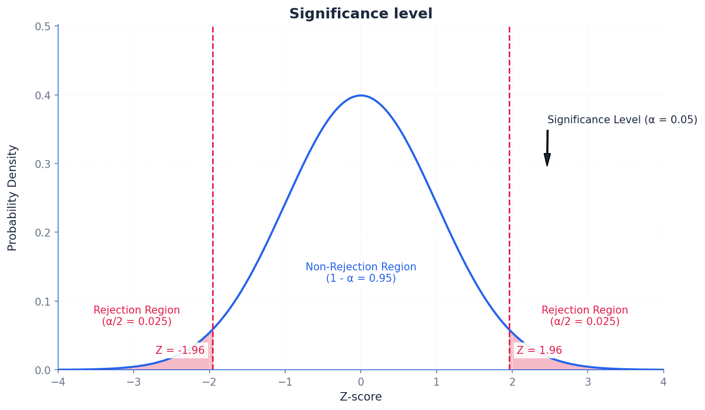
Students often think a 5% significance level means there's a 5% chance the alternative hypothesis is true, but actually it means there's a 5% chance of incorrectly rejecting a true null hypothesis.
Always state the chosen significance level (e.g., 5% or 0.05) at the beginning of your hypothesis test and use it consistently to compare with your calculated p-value or critical region.
test statistic — The test statistic is the calculated probability using sample data in a hypothesis test.
The test statistic is a value calculated from the sample data during a hypothesis test. This value is then compared to the critical region or used to find a p-value, which helps in deciding whether to reject or accept the null hypothesis. If you're testing a new recipe, the 'test statistic' is the taste score given by a sample of tasters. You compare this score to a benchmark to decide if the recipe is better.
Students often confuse the test statistic with the critical value, but actually the test statistic is calculated from the sample data, while the critical value is determined by the significance level and distribution.
critical region — The range of values at which you reject the claim is the critical region or rejection region.
The critical region is the set of values of the test statistic for which the null hypothesis is rejected. Its size is determined by the significance level, and it can be located in one tail (one-tailed test) or both tails (two-tailed test) of the distribution. Think of a target board. The bullseye is the 'acceptance region', but if your arrow lands outside a certain ring (the critical region), you 'reject' the idea that you hit the target accurately.
rejection region — The range of values at which you reject the claim is the critical region or rejection region.
The rejection region is another name for the critical region, representing the set of outcomes for which the null hypothesis is rejected. If the calculated test statistic falls within this region, the null hypothesis is rejected in favor of the alternative hypothesis. In a game, if your score falls into a certain 'danger zone' (rejection region), you lose. Otherwise, you continue playing (accept the null hypothesis).
Students often think the critical region is where the alternative hypothesis is true, but actually it's the region where the observed data is so extreme that it provides strong evidence against the null hypothesis.
Clearly define the critical region in terms of the test statistic (e.g., X ≤ 1 or X ≥ 12) and ensure it corresponds to the direction of the alternative hypothesis and the chosen significance level.
critical value — The value at which you change from accepting to rejecting the claim is the critical value.
The critical value is the boundary point(s) of the critical region. If the test statistic falls beyond this value (into the critical region), the null hypothesis is rejected. It is determined by the significance level and the distribution of the test statistic. Imagine a 'pass/fail' mark on an exam. If your score (test statistic) is below that mark (critical value), you fail (reject the null hypothesis).
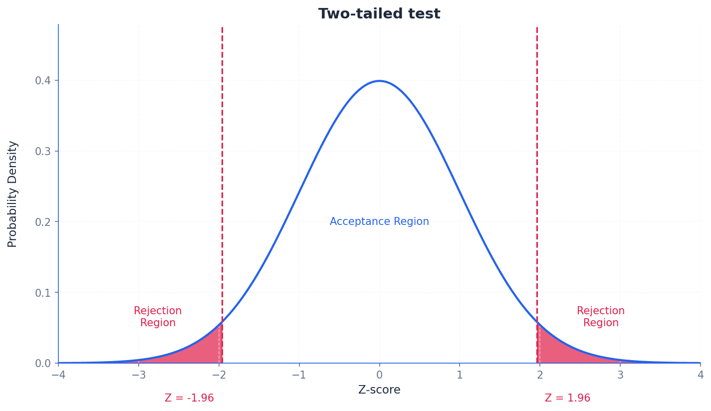
acceptance region — The other region of the graph is the acceptance region.
The acceptance region is the set of values of the test statistic for which the null hypothesis is not rejected. If the calculated test statistic falls within this region, there is insufficient evidence to reject the null hypothesis. If a product passes a quality check (its measurements fall within acceptable limits), it's in the 'acceptance region'. If it's outside, it's rejected.
Students often think 'accepting' the null hypothesis means it's proven true, but actually it just means there isn't enough evidence to reject it; it doesn't confirm its truth.
Hypothesis testing is a statistical method used to analyze data and draw conclusions about claims regarding a population parameter. It involves setting up two opposing statements: the null hypothesis (H0), which represents the status quo or no effect, and the alternative hypothesis (H1), which contradicts H0. The goal is to determine if there is sufficient evidence from sample data to reject H0 in favour of H1.
The nature of the alternative hypothesis determines whether a test is one-tailed or two-tailed. A one-tailed test is used when H1 specifies a direction (e.g., a probability is less than or greater than a certain value). A two-tailed test is used when H1 suggests a difference in either direction (e.g., a probability is not equal to a certain value). For two-tailed tests, the significance level is split equally between the two tails of the distribution.
Incorrectly choosing between a one-tailed and two-tailed test; the choice depends on whether the claim specifies a direction (increase/decrease) or just a difference.
When dealing with a single observation from a binomial distribution, hypothesis tests can be carried out using direct probability evaluation. This involves calculating the probability of observing the sample data (or more extreme data) under the assumption that the null hypothesis is true. This calculated probability, often referred to as the p-value, is then compared to the significance level to make a decision about H0.
For large sample sizes, a binomial distribution can be approximated by a normal distribution. This approximation simplifies calculations, especially when direct binomial probability evaluation becomes cumbersome. When using a normal approximation, it is crucial to apply a continuity correction to account for the discrete nature of the binomial distribution being approximated by a continuous normal distribution.
Forgetting to apply continuity correction when approximating a binomial distribution with a normal distribution.
Type I error — A Type I error occurs when a true null hypothesis is rejected.
A Type I error happens when the null hypothesis is true, but based on the sample data, we incorrectly reject it. The probability of making a Type I error is equal to the significance level (α) of the test. In a courtroom, a Type I error is when an innocent person is found guilty.
Type II error — A Type II error occurs when a false null hypothesis is accepted.
A Type II error happens when the null hypothesis is false, but based on the sample data, we incorrectly fail to reject it. The probability of making a Type II error is denoted by β and is harder to calculate as it depends on the true value of the population parameter under the alternative hypothesis. In a courtroom, a Type II error is when a guilty person is found innocent.
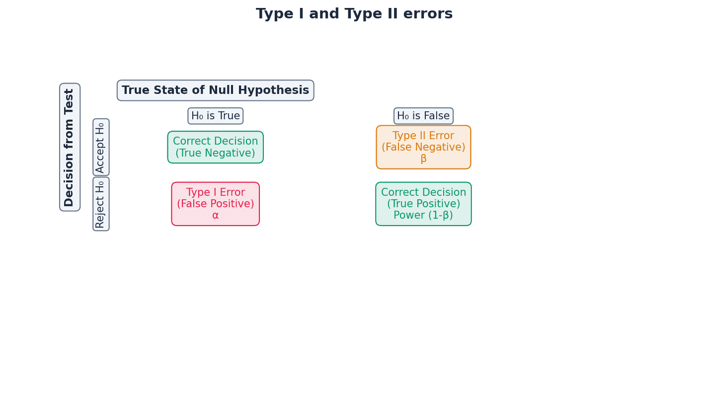
Confusing Type I and Type II errors, or their probabilities (significance level vs. beta).
When asked to explain a Type I error in context, state that it is concluding the alternative hypothesis is true when the null hypothesis is actually true, without using H0 or H1 in the explanation.
To calculate the probability of a Type II error, you need to assume a specific true value for the population parameter under the alternative hypothesis, which is often provided in the question.
Always state your null (H0) and alternative (H1) hypotheses clearly in terms of the population parameter (e.g., p).
Ensure your conclusion is stated in context, avoiding definitive language like 'proven' and instead using phrases like 'there is sufficient evidence to suggest...'.
When using a normal approximation, explicitly state the distribution used (e.g., X ~ N(np, npq)) and show the continuity correction.
Method Frameworks
Common Errors
| Common mistake | How to fix it |
|---|---|
| Confusing the null hypothesis with what the researcher wants to prove. | Remember H0 is the statement of no effect or no difference, which the researcher tries to disprove. |
| Incorrectly choosing between a one-tailed and two-tailed test. | The choice depends on whether the claim specifies a direction (e.g., 'less than', 'greater than') or just a general difference ('not equal to'). |
| Forgetting to apply continuity correction when using a normal approximation. | Always adjust the discrete value by ±0.5 when converting from a discrete (binomial) to a continuous (normal) distribution. |
| Interpreting 'accept H0' as proving H0 is true. | Phrase conclusions carefully: 'there is insufficient evidence to reject H0' rather than 'H0 is true'. |
| Confusing Type I and Type II errors or their probabilities. | Type I error is rejecting a true H0 (probability α). Type II error is accepting a false H0 (probability β). |
| Not stating conclusions in context or implying certainty. | Always relate your conclusion back to the original problem and use cautious language like 'there is sufficient evidence to suggest...'. |
Technique Selection
| When you see... | Use... |
|---|---|
| Small sample size (n) for binomial distribution, or when exact probabilities are required. | Direct probability evaluation using the binomial distribution (P(X=x) or cumulative P(X≤x)). |
| Large sample size (n) for binomial distribution (typically np > 5 and n(1-p) > 5). | Normal approximation to the binomial distribution, always with continuity correction. |
| Claim specifies a direction (e.g., 'less than', 'more than', 'decreased', 'increased'). | One-tailed hypothesis test. |
| Claim specifies a difference but no particular direction (e.g., 'different from', 'not equal to'). | Two-tailed hypothesis test (split significance level between tails). |
| Calculating the probability of rejecting a true null hypothesis. | Probability of Type I error (equal to the significance level α). |
| Calculating the probability of failing to reject a false null hypothesis (requires a specific true value for the alternative hypothesis). | Probability of Type II error (β). |
Mark Scheme Notes