A geometric shape undergoes two successive transformations in the coordinate plane. (a) Find the single matrix P representing a rotation of 45 degrees anticlockwise about the origin followed by an enlargement with scale factor $\sqrt{2}$ about the origin. [4] (b) Describe the single transformation represented by P. [4] (c) Compare the effect of applying the transformations in the reverse order. [4]

A geometric transformation maps points in the Cartesian plane. (a) Determine the matrix that represents a reflection in the line y = -x. [4] (b) Find the image of the line y = 2x + 1 under this transformation. [4] (c) Show that the line y = -x is an invariant line for this transformation. [3]

Shears are a type of linear transformation that distort a shape in a specific way while preserving its area. (a) State the matrix for a shear with the x-axis fixed and shear factor k. [2] (b) Describe the effect of a shear on the area of a shape. [3]

Consider the transformation represented by the matrix $\mathbf{M} = \begin{pmatrix} 1 & 0 \\ k & 1 \end{pmatrix}$, where $k$ is a non-zero constant. (a) Analyse the effect of applying this transformation to a general point $(x, y)$. [4] (b) Explain why this transformation is classified as a shear. [3] (c) Derive the equation of the fixed line for this shear. [3]

Transformations can be represented by matrices, and their effects can be observed by looking at how they map points or shapes. (a) Calculate the image of the point (2, 3) under a rotation of $60^\circ$ anticlockwise about the origin. [3] (b) Describe the transformation if the image of (1, 0) is (2, 0) and the image of (0, 1) is (0, 1). [3] (c) Draw the object and image for the transformation described in part (b) using the unit square as the object. [3]

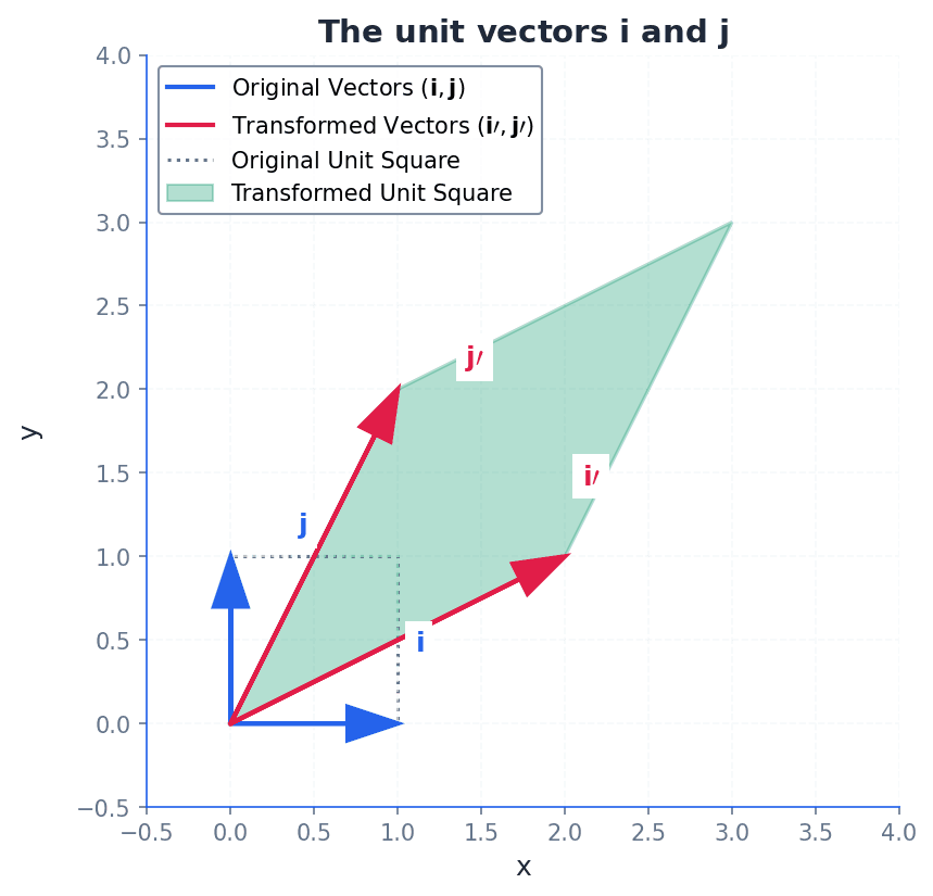
Fig 1.6 shows the unit vectors $\mathbf{i}$ and $\mathbf{j}$ and their images, $\mathbf{i}'$ and $\mathbf{j}'$, respectively, after a transformation. The unit square is transformed into the shaded region. (a) Describe fully the transformation represented by the matrix derived from Figure 1.6. (b) Calculate the determinant of the transformation matrix. (c) Find the area of the transformed unit square shown in Figure 1.6.

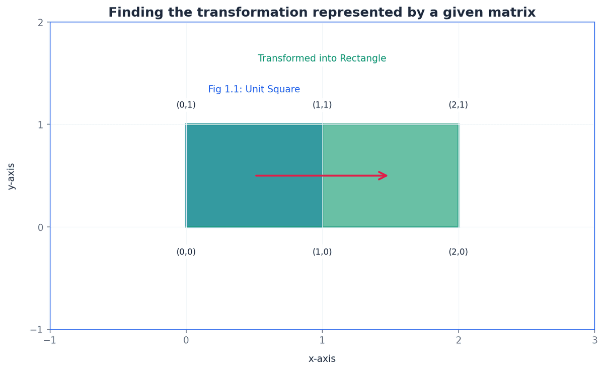
A unit square with vertices (0,0), (1,0), (1,1), (0,1) is transformed by a matrix M to produce an image. Fig 1.1 shows the object (unit square) and its image (a rectangle). (a) Identify the type of transformation represented by the matrix M shown in Fig 1.1. [3] (b) Determine the matrix M. [3] (c) Calculate the image of the point (3, 2) under this transformation. [2]

A triangle with vertices A(1,1), B(3,1), C(1,3) is transformed by a matrix M to produce an image triangle with vertices A'( -1, 1), B'( -1, 3), C'( -3, 1). Fig 1.2 shows the object triangle and its image triangle. (a) Describe the transformation represented by the matrix M shown in Fig 1.2. [4] (b) Find the matrix M. [4] (c) Determine the area of the image of a square of side length 2 units under this transformation. [3]

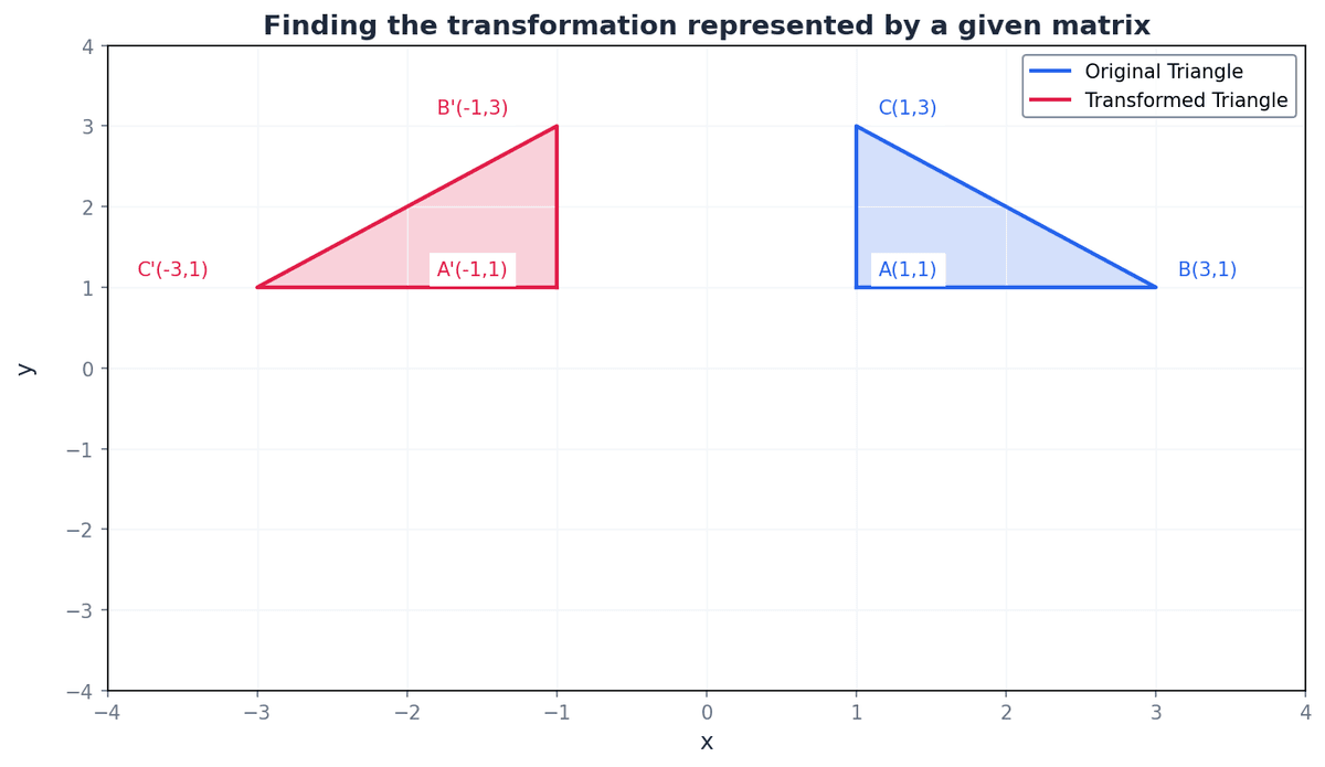
Fig 1.18 illustrates successive transformations A and B on a point P(1,2). P is mapped to A(P), and A(P) is then mapped to B(A(P)). (a) Describe the transformation A that maps P to A(P). (b) Describe the transformation B that maps A(P) to B(A(P)). (c) Determine the matrix BA and calculate the image of the point (3,4) under this composite transformation.

Transformations can be applied to points and shapes using matrix multiplication. Consider an enlargement transformation. (a) Find the matrix that represents an enlargement, centre the origin, with scale factor 3. [3] (b) Calculate the image of the point (2, -1) under this enlargement. [4]

Fig 1.7 shows the unit vectors i and j, and their images i' and j' after a transformation. The original unit square has vertices (0,0), (1,0), (1,1), (0,1). The transformed unit square has vertices (0,0), (0,1), (1,1), (1,0). (a) Describe fully the transformation represented by the matrix derived from Fig 1.7. (b) Calculate the determinant of the transformation matrix. (c) Find the equation of the invariant line for this transformation. Explain why this line is invariant.

Fig 1.3 shows a transformation of an object triangle ABC to its image A'B'C'. (a) Identify the coordinates of the vertices of the object triangle ABC from Fig 1.3. (b) Calculate the midpoint of side AB for the object triangle ABC. (c) Sketch the image of this midpoint under the transformation and state its coordinates.

The rotation matrix provides a powerful tool for linking geometric transformations with trigonometric identities. (a) Derive the matrix for a rotation of angle A anticlockwise about the origin. [4] (b) By considering the product of two rotation matrices, prove the trigonometric identity for sin(A+B). [4]

A transformation is represented by the shear matrix M = \begin{pmatrix} 1 & k \\ 0 & 1 \end{pmatrix}. (a) Show that the line y=mx is an invariant line for this shear if m=0. [3] (b) Determine the invariant points for the shear represented by M = \begin{pmatrix} 1 & 3 \\ 0 & 1 \end{pmatrix}. [4] (c) Find the equation of the invariant line for the shear given in part (b). [3]

A shear transformation is applied to points in the Cartesian plane. The x-axis remains fixed, and the point (0, 1) is mapped to (4, 1). (a) Find the matrix that represents this shear. [5] (b) Show the effect of this shear on a rectangle with vertices (0,0), (2,0), (2,3), (0,3) by drawing the object and its image on a coordinate grid. [4]

A geometric transformation reflects points in a line passing through the origin. Consider the line $y = (\tan \theta) x$, which makes an angle $\theta$ with the positive x-axis. (a) Derive the matrix that represents a reflection in the line $y = (\tan \theta) x$. [5] (b) Show that for $\theta = 45^\circ$, your derived matrix matches the standard reflection matrix in $y=x$. [4] (c) Calculate the image of the point (1, 0) under a reflection in the line $y = \sqrt{3} x$. [3]

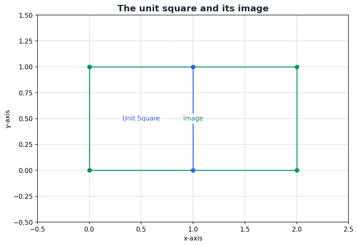
Fig 1.12 shows the unit square and its image after a transformation. (a) Describe fully the transformation shown in Figure 1.12. (b) Calculate the determinant of the transformation matrix from Figure 1.12. (c) Find the image of the point (-2,3) under this transformation.

Rotations are a common type of transformation that can be represented by a matrix. (a) Describe the transformation represented by the matrix $\begin{pmatrix} \cos(90^\circ) & -\sin(90^\circ) \\ \sin(90^\circ) & \cos(90^\circ) \end{pmatrix}$. [4] (b) Show the effect of this transformation on the unit square by drawing the object and its image on a coordinate grid. [4]

A unit square has vertices at (0,0), (1,0), (1,1) and (0,1). (a) Draw the image of the unit square under the transformation represented by \begin{pmatrix} 1 & 0 \\ 0 & -1 \end{pmatrix}. [4] (b) Describe this transformation fully. [3]

Fig 1.18 illustrates successive transformations A and B on a point P(1,2). (a) Determine the matrix M_A that represents the transformation A from Fig 1.18. (b) Find the inverse matrix M_A^(-1). (c) Apply M_A^(-1) to the point A(P) and state the result.

Geometric transformations can be represented by matrix multiplication, mapping an object to its image. Fig 1.1 shows a triangle PQR and its image P'Q'R' after a transformation. (a) Analyse the transformation applied to the triangle PQR to obtain P'Q'R' as shown in Fig 1.1, and determine the transformation matrix M. [6] (b) Compare the area of triangle PQR with the area of triangle P'Q'R' and deduce the scale factor of the transformation from the determinant of M. [6]

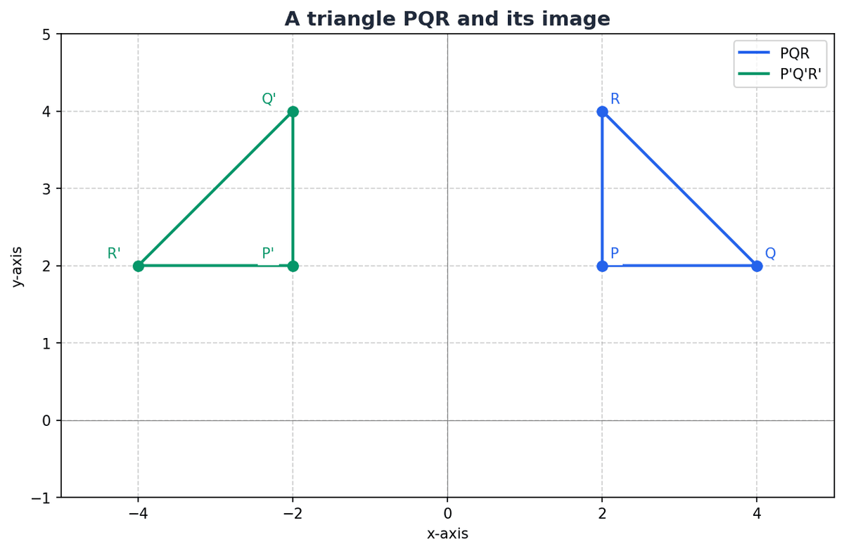
Fig 1.1 shows direct flights between countries by one airline. (a) Construct the adjacency matrix M for the flight network shown in Figure 1.1, where M_ij = 1 if there is a direct flight from country i to country j, and 0 otherwise. Use the order Philippines, Singapore, Australia, New Zealand, UK. (b) Calculate the matrix M^2. (c) Interpret the element in the third row, fifth column of M^2 in the context of flight paths.

Fig 1.18 illustrates successive transformations A and B on a point P(1,2). (a) Determine the matrix M_A that represents the transformation A in Figure 1.18. [3] (b) Find the matrix M_B that represents the transformation B in Figure 1.18. [3] (c) Show that the transformation A is a rotation about the origin. Calculate the angle of rotation. Show that the transformation B is a reflection. State the line of reflection. [6]

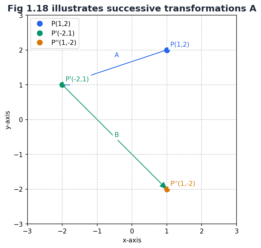
Fig 1.12 shows the unit square and its image after a transformation. (a) State the coordinates of the unit vectors I and J from Figure 1.12. (b) Write down the image coordinates I' and J' after the transformation. (c) Calculate the transformation matrix M based on I' and J'.

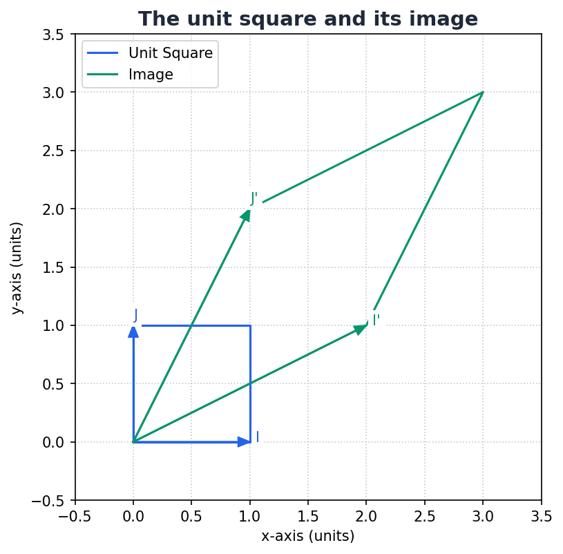
Fig 1.15 shows the unit square and its image under a shear transformation. (a) State the coordinates of the original unit vectors $\mathbf{i}$ and $\mathbf{j}$ from Figure 1.15. (b) Find the images of the unit vectors $\mathbf{i}$ and $\mathbf{j}$ after the shear transformation shown in Figure 1.15. (c) Determine the matrix that represents this shear transformation, using the images of the unit vectors.

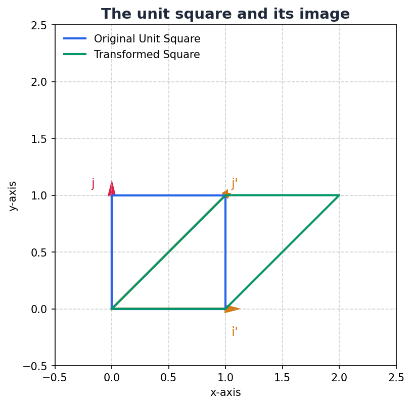
Fig 1.15 shows the unit square and its image under a shear transformation. (a) Identify the fixed line for the shear transformation shown in Figure 1.15. (b) Determine the shear factor $k$ for this transformation, by observing the coordinates of the image of the point (0,1). (c) Calculate the matrix that represents this shear transformation. (d) Explain why the area of the transformed unit square is equal to the area of the original unit square.

A shear transformation, S, has the y-axis as its fixed line. This means that points on the y-axis remain unchanged, and other points move parallel to the y-axis. (a) Find the matrix for a shear with the y-axis fixed such that the point (2, 1) maps to (2, 7). [4] (b) Calculate the image of the point (5, -3) under this shear. [4]

A point in the Cartesian plane undergoes a sequence of transformations. (a) Calculate the single matrix representing a stretch of factor 3 parallel to the x-axis followed by a shear with the y-axis fixed and shear factor 2. [4] (b) Describe the transformation represented by this single matrix. [4]

A linear transformation is defined by the matrix $\mathbf{M} = \begin{pmatrix} 4 & -2 \\ 2 & 0 \end{pmatrix}$. (a) Show that the transformation represented by $\mathbf{M}$ has exactly two distinct invariant lines, and find their equations. [7] (b) Deduce the intersection point of these two invariant lines. [2]

Matrices are fundamental tools in mathematics, used to represent linear transformations and solve systems of equations. Unlike scalar multiplication, the order of matrix multiplication is crucial. (a) For the matrices $\mathbf{P} = \begin{pmatrix} 2 & -1 \\ 3 & 4 \end{pmatrix}$ and $\mathbf{Q} = \begin{pmatrix} 1 & 0 \\ -2 & 5 \end{pmatrix}$, show that $\mathbf{P}\mathbf{Q} \ne \mathbf{Q}\mathbf{P}$. [6] (b) Deduce what this implies about matrix multiplication in general. [4]

Fig 1.7 shows the unit vectors i and j, and their images i' and j' after a transformation. The original unit square has vertices (0,0), (1,0), (1,1), (0,1). The transformed unit square has vertices (0,0), (0,1), (1,1), (1,0). (a) Identify the coordinates of the origin O and the unit vectors i and j from Fig 1.7. (b) Calculate the image of the unit vectors i and j after the transformation shown in Fig 1.7. (c) Determine the matrix that represents this transformation.

A transformation is represented by the matrix T = \begin{pmatrix} 1 & a \\ 2 & 3 \end{pmatrix}, where 'a' is a constant. (a) Determine the values of the constant 'a' for which this transformation has only one invariant line. Find the equation of this invariant line for these values of 'a'. [8] (b) Explain the geometrical significance of having only one invariant line. [2]

Transformations are a fundamental concept in linear algebra, mapping points or shapes from one position to another. (a) Define what is meant by a 'linear transformation'. [2] (b) Give two properties that are preserved under a linear transformation. [3]

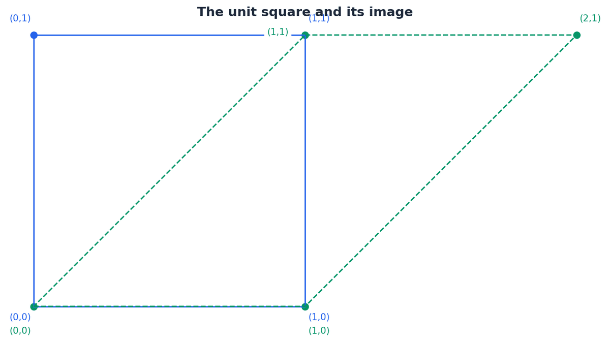
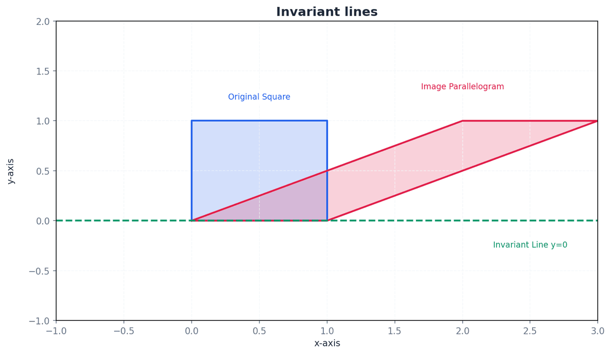
Fig 1.1 shows the unit square (with vertices at (0,0), (1,0), (1,1), (0,1)) and its image after transformation by the matrix M = \begin{pmatrix} 1 & 2 \\ 0 & 1 \end{pmatrix}. (a) Identify the invariant lines for the transformation represented by M from Fig 1.1. Write down their equations. [5] (b) Illustrate how a point on one of these invariant lines moves under the transformation M, by choosing a specific point and its image from the diagram. [3]

Matrix multiplication is a key operation in linear algebra, but it has specific rules regarding when it can be performed. (a) Calculate the product $\mathbf{A}\mathbf{B}$ for $\mathbf{A} = \begin{pmatrix} 4 & 1 \\ 2 & 3 \end{pmatrix}$ and $\mathbf{B} = \begin{pmatrix} 5 \\ -2 \end{pmatrix}$. [4] (b) Determine if $\mathbf{B}\mathbf{A}$ is conformable for multiplication, explaining your reasoning. [4]

Matrix multiplication has specific rules regarding the order and dimensions of matrices. Consider two matrices, P and Q. (a) Give an example of two 2x2 matrices, P and Q, such that PQ is defined. [2] (b) Identify the order of the product PQ. [2]

Fig 1.20 shows a reflection in the line l. Point P(2,1) is reflected to P'(1,2). The line l passes through Q(3,3) and R(0,0). (a) Determine the matrix M for the reflection shown in Fig 1.20. (b) Find the equation of the line perpendicular to l that passes through P(2,1). (c) Show that the line found in part (b) is an invariant line under the transformation M, by taking a general point on this line and showing its image also lies on the same line.

Given the matrices $\mathbf{A} = \begin{pmatrix} 3 & 2 \\ -1 & 5 \end{pmatrix}$ and $\mathbf{B} = \begin{pmatrix} 0 & -4 \\ 6 & 1 \end{pmatrix}$. (a) Calculate $\mathbf{A} + \mathbf{B}$. [3] (b) Calculate $2\mathbf{A}$. [3]

In the study of matrix transformations, certain geometric features remain unchanged. These are often referred to as invariant properties. (a) Define the term 'invariant line' in the context of matrix transformations. [2] (b) State the general approach to finding invariant lines for a given 2x2 matrix transformation. [3]

Transformations can map points from one position to another. Sometimes, a point remains in its original position after a transformation. (a) Define what is meant by an invariant point under a transformation. [2] (b) Find the invariant point for the transformation represented by the matrix $\begin{pmatrix} 1 & 0 \\ 0 & -1 \end{pmatrix}$. [3]