Nexelia Academy · Official Revision Notes
Complete A-Level revision notes · 7 chapters
This chapter introduces matrices as rectangular arrays of numbers, defining their order and special types. It covers fundamental matrix operations and explores how matrices represent 2D geometric transformations. Finally, it discusses successive transformations, invariant points, and invariant lines.
matrix — A matrix is an array of numbers, usually written inside curved brackets.
Matrices are used to represent data or transformations. They consist of rows and columns, with individual entries called elements. Think of a matrix like a spreadsheet or a grid of numbers, where each cell holds a specific value and its position matters.
elements — The entries in the various cells of a matrix are known as elements.
Each number or variable within a matrix is an element. Their position within the matrix (row and column index) is important for matrix operations and defining the matrix's order. If a matrix is a bookshelf, then each book on the shelf is an element.
order — The order of a matrix is stated by the number of rows first, then the number of columns.
For example, a 5 × 5 matrix has five rows and five columns. The order is fundamental as it determines whether matrices can be added, subtracted, or multiplied. The order of a matrix is like the dimensions of a room – length by width.
Always state the order correctly as 'rows × columns'; reversing this will lose marks, especially in questions about conformability.
square matrices — Matrices that have the same number of rows as columns are called square matrices.
Examples include 2 × 2 or 3 × 3 matrices. Square matrices are important for operations like finding determinants, inverses, and representing certain transformations. A square matrix is like a square grid or a chessboard, where the number of rows equals the number of columns.
identity matrix — An identity matrix is a square matrix with 1s on the leading diagonal and zeros elsewhere, usually denoted by I.
When an identity matrix multiplies another matrix, the other matrix remains unchanged, similar to how multiplying a number by 1 leaves it unchanged. Identity matrices must be square. The identity matrix is like the number '1' in scalar multiplication; it leaves the other matrix unchanged when multiplied.
unit matrix — The unit matrix is another name for the identity matrix.
It serves the same purpose as the identity matrix, leaving other matrices unchanged upon multiplication. It is always a square matrix with ones on the main diagonal and zeros elsewhere. Just like a 'unit' of measurement is a standard, the unit matrix is the standard 'multiplicative identity' for matrices.
Remember that I can be of any square order (e.g., I₂ or I₃) and its specific order is usually implied by the context of the multiplication.
zero matrix — A zero matrix is a matrix where all elements are zero, usually denoted by O.
When a zero matrix is added to another matrix, the other matrix remains unchanged, similar to how adding 0 to a number leaves it unchanged. Zero matrices can be of any order. The zero matrix is like the number '0' in scalar addition; it leaves the other matrix unchanged when added.
equal matrices — Two matrices are said to be equal if, and only if, they have the same order and each element in one matrix is equal to the corresponding element in the other matrix.
This means that for matrices A and B to be equal, they must have the same number of rows and columns, and aᵢⱼ must equal bᵢⱼ for all i and j. Two matrices being equal is like having two identical jigsaw puzzles; they must have the same number of pieces (order) and each piece must match its corresponding piece in the other puzzle (elements).
Matrices can be added or subtracted if they have the same order. This involves adding or subtracting corresponding elements. If matrices are not of the same order, they are non-conformable for addition, and the operation is undefined. Scalar multiplication involves multiplying every element within a matrix by a single number, called a scalar, which changes the magnitude of the elements but not the matrix's order.
non-conformable for addition — Matrices are non-conformable for addition if they are not of the same order.
Matrix addition and subtraction require matrices to have identical dimensions (same number of rows and columns) because elements are added or subtracted in corresponding positions. Trying to add non-conformable matrices is like trying to add apples and oranges; they are different types of items and cannot be combined directly.
scalar number — A scalar number is a single number by which a matrix can be multiplied.
When a matrix is multiplied by a scalar, every element within the matrix is multiplied by that scalar. This operation changes the magnitude of the matrix elements but not its order. Multiplying a matrix by a scalar is like scaling a recipe; if you double the recipe (scalar factor of 2), you double every ingredient (element).
Students often think scalar multiplication only applies to certain elements, but actually it applies to every single element in the matrix.
Matrix multiplication is a more complex operation than addition or scalar multiplication. Two matrices are conformable for multiplication if the number of columns in the first matrix equals the number of rows in the second matrix. The resulting product matrix will have an order determined by the outer dimensions of the original matrices. Each element of the product is found by multiplying elements of a row from the first matrix by elements of a column from the second matrix and summing the products.
conformable for multiplication — Two matrices are conformable for multiplication if the number of columns in the first matrix equals the number of rows in the second matrix.
For matrices A (order m × n) and B (order n × p), the product AB exists because the 'middle' numbers (n) are the same. The resulting product matrix will have the order m × p. Being conformable for multiplication is like connecting two gears; the number of teeth on the output of the first gear must match the number of teeth on the input of the second gear for them to mesh.
Matrix Multiplication (2x2)
The product of a 2x2 matrix with another 2x2 matrix results in a 2x2 matrix. Each element of the product is found by multiplying elements of a row from the first matrix by elements of a column from the second matrix and summing the products.
Students often think any two matrices can be multiplied, but actually they must be conformable for multiplication (inner dimensions must match).
Always write down the orders of the matrices (e.g., 2×4 and 4×1) to visually check if the inner numbers match and to determine the order of the product matrix.
Matrix multiplication is associative, meaning (AB)C = A(BC). However, it is generally not commutative, so AB ≠ BA. This non-commutativity is a crucial distinction from scalar multiplication and has significant implications when dealing with successive transformations. The identity matrix, I, acts as the multiplicative identity, such that AI = IA = A.
Students often think matrix multiplication is commutative (AB = BA), but actually it is generally not commutative.
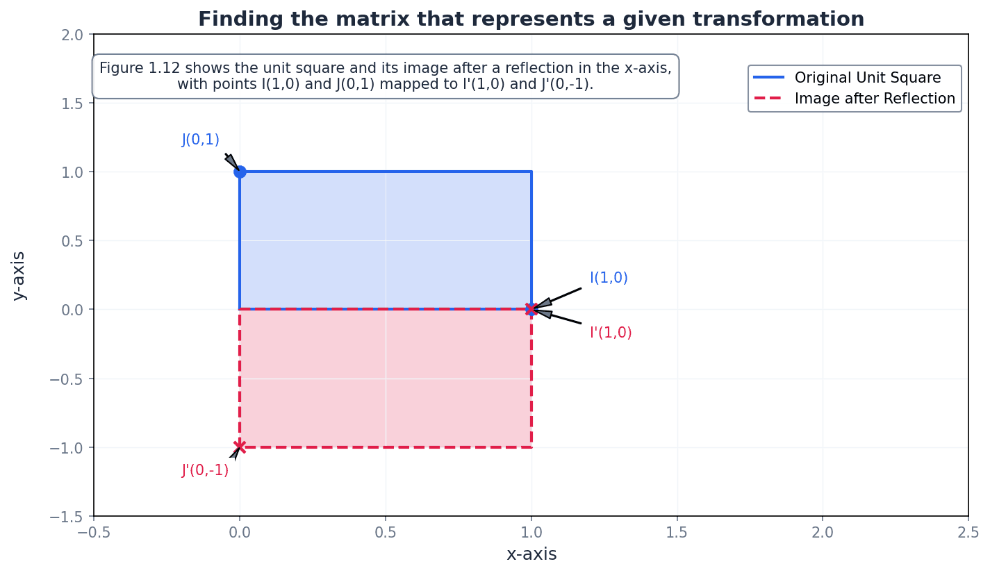
Matrices are powerful tools for representing 2D geometric transformations in the x-y plane. A transformation is a mapping of an object (the original point or shape) onto its image (the new point or shape). All transformations represented by matrices are linear transformations, meaning straight lines map to straight lines and the origin maps to itself. Unit vectors, i = (1, 0) and j = (0, 1), are fundamental for finding transformation matrices, as their images under a transformation form the columns of the matrix.
object — The original point, or shape, before a transformation is called the object.
In geometric transformations, the object is the starting figure. Its coordinates or shape are altered by the transformation to produce the image. The object is like the original photograph before you apply any filters or edits.
image — The new point, or shape, after the transformation, is called the image.
The image is the result of applying a transformation to an object. Its position, orientation, or size may differ from the original object. The image is like the edited photograph after you've applied filters or made changes.
transformation — A transformation is a mapping of an object onto its image.
Transformations describe how points or shapes move in a coordinate system. They can be represented by matrices and include reflections, rotations, enlargements, stretches, and shears. A transformation is like a set of instructions for moving or changing a piece on a chessboard; it tells you exactly where the piece ends up.
unit vectors — Vectors that have length or magnitude of 1 are called unit vectors.
In two dimensions, i = (1, 0) and j = (0, 1) are unit vectors along the x-axis and y-axis, respectively. Their images under a transformation matrix form the columns of that matrix. Unit vectors are like the basic building blocks or fundamental directions (north, east) in a coordinate system, each having a standard length of one step.
Remember that the images of i and j directly give the columns of the transformation matrix; this is a quick way to find the matrix for a given transformation.
linear transformations — In a linear transformation, straight lines are mapped to straight lines, and the origin is mapped to itself.
All transformations represented by matrices (reflections, rotations, enlargements, stretches, shears) are examples of linear transformations. This property ensures that the 'straightness' of objects is preserved. A linear transformation is like drawing on a rubber sheet that you can stretch or twist, but you can't tear it or fold it over itself; straight lines remain straight.
If a transformation does not map the origin to itself, it cannot be represented by a 2x2 matrix and is not a linear transformation.
Various geometric transformations can be represented by specific 2x2 matrices. These include rotations about the origin, reflections in standard lines (x-axis, y-axis, y=x, y=-x), enlargements centered at the origin, stretches parallel to an axis, and shears. Understanding how these matrices are derived, often by observing the images of the unit vectors, is key to both describing and finding transformation matrices.
Rotation matrix (anticlockwise about origin)
This matrix transforms a point (x, y) to its image (x', y') after an anticlockwise rotation of angle θ about the origin.
Stretch parallel to x-axis
This matrix represents a stretch of scale factor m parallel to the x-axis. The y-coordinates remain unchanged.
Stretch parallel to y-axis
This matrix represents a stretch of scale factor n parallel to the y-axis. The x-coordinates remain unchanged.
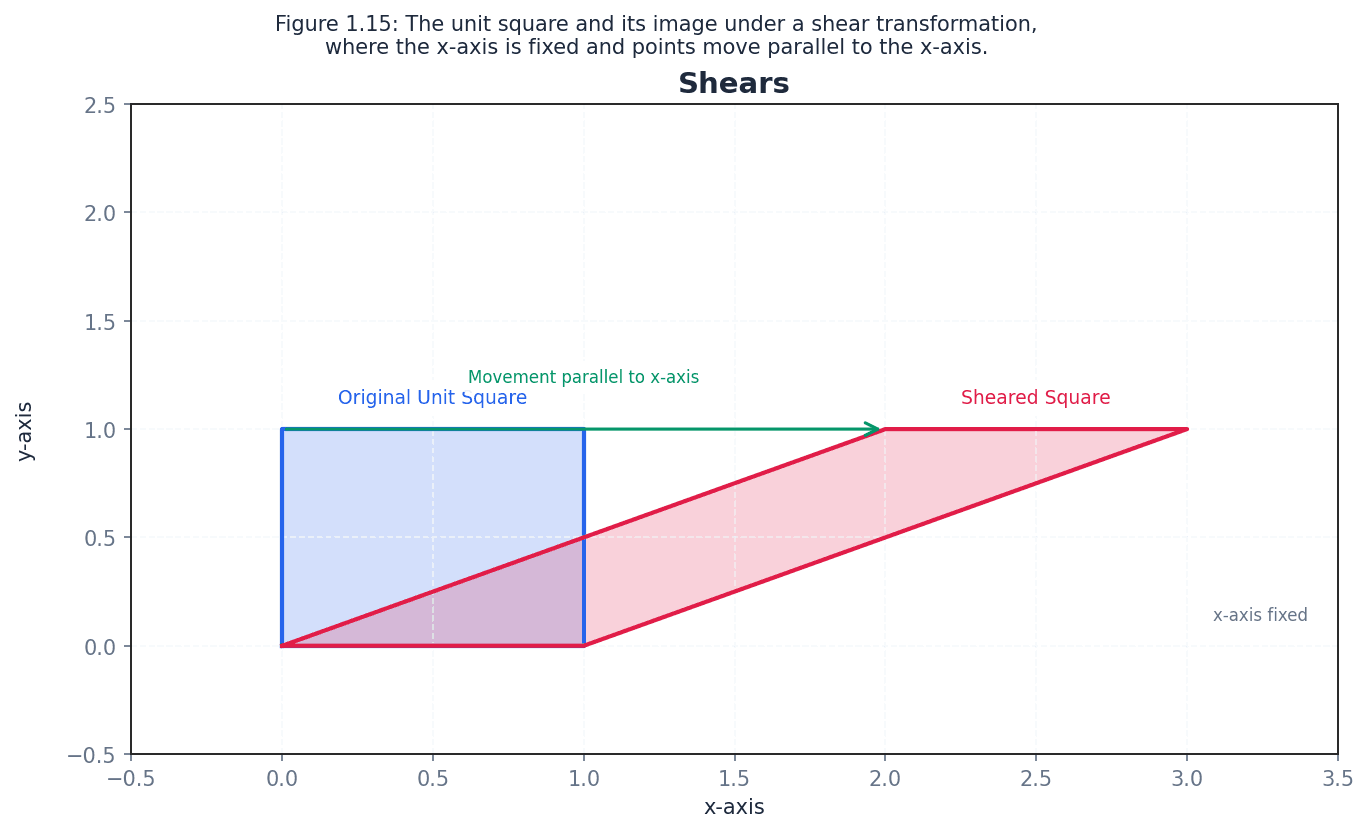
Shear (x-axis fixed)
This matrix represents a shear with the x-axis fixed. Points move parallel to the x-axis.
Shear (y-axis fixed)
This matrix represents a shear with the y-axis fixed. Points move parallel to the y-axis.
shear — A shear is a transformation where points on a fixed line stay the same, and other points move parallel to the fixed line by a distance proportional to their perpendicular distance from the fixed line.
For example, a shear with the x-axis fixed transforms the unit vector j=(0,1) to (k,1), where k is the shear factor. It distorts shapes, turning rectangles into parallelograms. Imagine pushing the top of a stack of cards while keeping the bottom card fixed; the cards slide past each other, creating a slanted stack. This is similar to a shear.
When describing a shear, always state the fixed line (e.g., x-axis fixed) and the image of a point not on the fixed line (e.g., (0,1) mapped to (k,1)).
Reflection in x-axis
This matrix reflects a point across the x-axis.
Reflection in y-axis
This matrix reflects a point across the y-axis.
Reflection in line y=x
This matrix reflects a point across the line y=x.
Reflection in line y=-x
This matrix reflects a point across the line y=-x.
Enlargement (centre origin, scale factor k)
This matrix represents an enlargement with the origin as the centre and a scale factor of k.
When multiple transformations are applied one after another, they form a successive transformation. The composite transformation matrix is found by multiplying the individual transformation matrices. Crucially, if transformation B is followed by transformation A, the composite matrix is AB. The order of matrix multiplication is vital here due to its non-commutative nature.
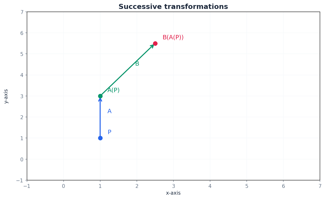
Students often reverse the order of transformations when forming a composite matrix (e.g., for B followed by A, they might write BA instead of AB). Remember that the matrix product AB represents the transformation B followed by A.
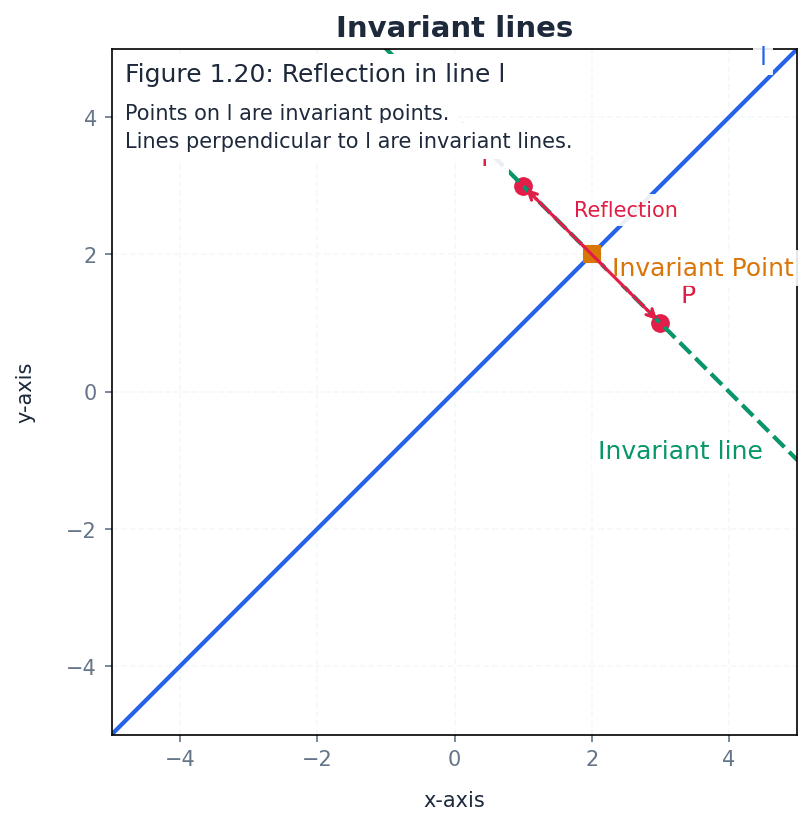
For any transformation, certain points or lines may remain unchanged. Points that map to themselves under a transformation are called invariant points. The origin (0,0) is always an invariant point for transformations represented by matrices. An invariant line is a line where the image of every point on that line is also on the same line, though not necessarily the same point.
invariant points — Points that map to themselves under a transformation are called invariant points.
For a point (x, y) to be invariant under a transformation represented by matrix M, M(x, y) must equal (x, y). The origin (0,0) is always an invariant point for transformations represented by matrices. An invariant point is like a pivot in a rotation; it's the only point that doesn't move.
To find invariant points, set M(x, y) = (x, y) and solve the resulting simultaneous equations. If the equations are equivalent, there is a line of invariant points.
invariant line — A line AB is known as an invariant line under a transformation if the image of every point on AB is also on AB.
It is not necessary for each point on the line to map to itself; it can map to another point on the same line. For example, in a reflection, the mirror line is an invariant line of invariant points, while lines perpendicular to the mirror line are invariant lines but not lines of invariant points. An invariant line is like a track on which a train moves; the train (point) moves, but it stays on the track (line).
Students often confuse invariant lines with lines of invariant points, but actually an invariant line only requires points to map to other points on the same line, not necessarily to themselves.
To find invariant lines, assume the line has the form y = mx + c (or x=k) and apply the transformation, then equate the image line to the original line to solve for m and c.
Use your calculator for matrix operations (addition, subtraction, multiplication) to save time and reduce errors in exams.
Exam Technique
Performing matrix multiplication
Finding the matrix for a given 2D transformation
| Mistake | Fix |
|---|---|
| Assuming matrix multiplication is commutative (AB = BA). | Always remember that matrix multiplication is generally not commutative. The order matters significantly, especially for successive transformations. |
| Attempting to multiply non-conformable matrices. | Before multiplying, always check that the number of columns in the first matrix equals the number of rows in the second matrix. If not, the multiplication is undefined. |
| Reversing the order of matrices for successive transformations. | For transformation B followed by A, the composite matrix is AB. The transformation applied first is on the right. |
This chapter introduces sequences and series, their notation, and various definitions. It covers methods for summing series, including standard formulae and the method of differences, culminating in a detailed explanation of proof by mathematical induction.
Sequence — A sequence is an ordered set of objects with an underlying rule.
Sequences can be defined inductively (term-to-term) or deductively (position-to-term). They can be increasing, decreasing, oscillating, or convergent, much like a list of instructions where each step depends on the previous one or its position.
Series — A series is the sum of the terms of a numerical sequence.
Series are often represented using sigma (Σ) notation, indicating the sum of terms from a specified starting limit to an ending limit. The sum can be finite or infinite, similar to adding up scores from each round of a game to get a total.
Students often confuse 'sequence' (an ordered list of terms) with 'series' (the sum of those terms). Remember that a sequence is the ordered list, while a series is the sum.
Inductive definition — An inductive definition describes the relationship between one term and the next in a sequence.
This type of definition requires a starting term (e.g., u1) and a rule to generate subsequent terms (e.g., ur+1 = ur + 3). It is also known as a term-to-term definition, acting like a chain reaction where each event triggers the next.
When asked for an inductive rule, ensure you provide both the first term (e.g., u1) and the recurrence relation (e.g., ur+1 = ...). Forgetting the starting term is a common error.
Deductive definition — A deductive definition describes the relationship between a term and its position in a sequence.
This definition allows you to directly calculate any term in the sequence by knowing its position (r), without needing to know the previous terms. It is also known as a position-to-term definition, like a formula that directly tells you the value of an item based on its slot number.
Increasing sequence — In an increasing sequence, each term is greater than the previous term.
For example, 2, 5, 8, 11, 14 is an increasing sequence because each term is larger than the one before it, implying a positive difference between consecutive terms. This is like climbing a staircase where each step is higher than the last.
Decreasing sequence — In a decreasing sequence, each term is smaller than the previous term.
For example, 14, 11, 8, 5, 2 is a decreasing sequence because each term is smaller than the one before it, implying a negative difference between consecutive terms. This is like walking downhill where each step takes you to a lower elevation.
Oscillating sequence — In an oscillating sequence, the terms lie above and below a middle number.
The terms do not consistently increase or decrease but rather alternate in value, often around a central point, such as 5, -5, 5, -5, ... This is like a pendulum swinging back and forth.
Convergent sequence — The terms of a convergent sequence get closer and closer to a limiting value.
As the number of terms (n) approaches infinity, the terms of the sequence approach a specific finite value, known as the limit. This is similar to a car slowing down as it approaches a stop sign, getting closer to a final position.
Sum of the first n integers
Used for summing consecutive positive integers starting from 1.
Sum of a constant
Used when summing a constant value 'c' n times.
Sum of the squares of the first n integers
Used for summing the squares of consecutive positive integers starting from 1.
Sum of the cubes of the first n integers
Used for summing the cubes of consecutive positive integers starting from 1.
Many series can be summed efficiently by applying standard formulae for the sum of the first n integers (Σr), squares (Σr²), and cubes (Σr³). These formulae allow for direct calculation of the sum without needing to list all terms. When dealing with sums involving constants or combinations of powers of r, the linearity of summation can be used to break down the problem into simpler parts, as seen in Example 2.3 and 2.4.
When using standard sum formulae, ensure you substitute 'n' correctly and simplify the resulting expression fully. Pay close attention to the limits of the sum in sigma notation; a common error is to sum over the wrong range of terms.
Method of differences — The method of differences is a technique to find the sum of a series by expressing each term as the difference of two (or more) terms from a related series, leading to cancellation.
This method is particularly effective when most intermediate terms cancel out, leaving only a few terms at the beginning and end of the series. This is often called a telescoping sum, much like a collapsible telescope where inner sections disappear, leaving only the end pieces.
Telescoping sum — A telescoping sum is a sum where most of the terms cancel out, leaving only the first and last few terms.
This occurs when each term in the series can be written as the difference of two consecutive terms of another sequence, such as f(r) - f(r-1). It's like a stack of cups where only the top and bottom are visible when pushed together.
For method of differences questions, clearly write out the first few and last few terms to demonstrate cancellation and identify remaining terms. Lay out the terms vertically to clearly see the cancellation pattern.
Students often struggle with setting up the terms correctly for cancellation in the method of differences. Careful layout of the terms in columns helps visualize which parts cancel, and it's important to identify all terms that do not cancel, not just pairwise ones.
For a convergent series, where the terms of the sequence get closer and closer to a limiting value, it is possible to find the sum to infinity. This is achieved by first finding the sum to n terms (S_n) and then evaluating the limit of S_n as n approaches infinity. If the terms involving n in the denominator tend to zero, the sum to infinity will be a finite constant, as demonstrated in Examples 2.7 and 2.8.
Proof by mathematical induction — Proof by mathematical induction is a method used to prove that a statement is true for all positive integers.
It involves two main steps: proving the base case (e.g., n=1) and proving the inductive step (if true for n=k, then true for n=k+1). Once these are established, the statement is true for all subsequent integers, much like climbing a ladder where you must get on the bottom rung and then be able to get from any rung to the next.
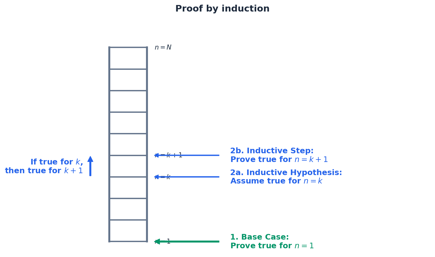
A proof by mathematical induction requires a clear structure. First, establish the base case, typically by showing the statement holds for n=1. Second, assume the statement is true for some positive integer k (the inductive hypothesis). Third, use this assumption to prove that the statement must also be true for n=k+1 (the inductive step). Finally, conclude that the statement is true for all positive integers by mathematical induction.
Students often assume the inductive step alone proves the statement, but actually it only proves 'if true for k, then true for k+1'. The base case is essential to start the chain of proof. Omitting the base case or the concluding statement invalidates the entire proof.
In proof by induction, clearly state the three steps: Base Case, Inductive Hypothesis (assume true for n=k), and Inductive Step (prove true for n=k+1). Always include a clear concluding statement, e.g., 'Therefore, by mathematical induction, the statement is true for all positive integers n'.
Pay close attention to the question's wording; 'find the sum' implies a numerical answer, while 'prove' requires a formal argument, often by induction.
Exam Technique
Finding the sum of a series using standard formulae
Finding the sum of a series using the method of differences
| Mistake | Fix |
|---|---|
| Confusing 'sequence' with 'series'. | Remember: a sequence is an ordered list of terms, while a series is the sum of those terms. |
| Forgetting to state the starting term (u1) in an inductive definition. | An inductive definition requires both the first term and the recurrence relation to uniquely define the sequence. |
| Incorrectly applying summation limits in sigma notation. | Always double-check the starting and ending values of 'r' in the sigma notation to ensure you are summing the correct range of terms. |
This chapter introduces polynomials, defining their order and the concept of roots, including real, complex, and repeated roots. It details the relationships between the roots and coefficients of quadratic, cubic, and quartic equations, known as Vieta's Formulae. The chapter also covers methods for forming new equations with roots related to a given equation's roots, and the evaluation of symmetric functions of roots.
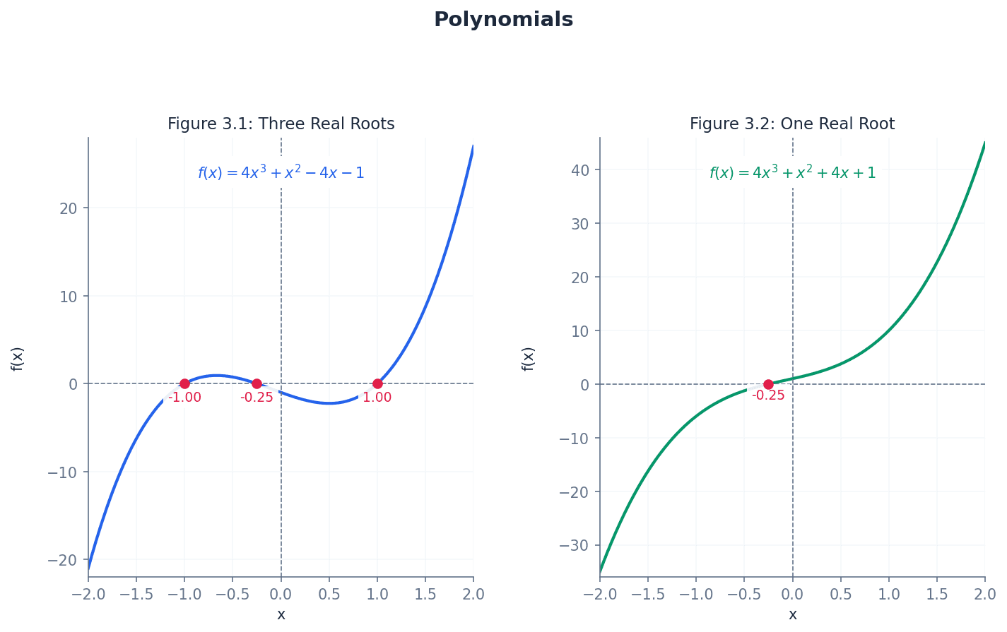
Polynomial — A polynomial is an expression like 4x³ + x² − 4x − 1, whose terms are all positive integer powers of a variable or multiples of them.
Polynomials are fundamental algebraic expressions, characterized by having only non-negative integer exponents for their variables. They do not contain square roots or reciprocals of variables, simplifying their analysis compared to more complex functions. Think of a polynomial as a 'building block' expression in algebra, made only from whole number powers of a variable, like building with Lego bricks where each brick is a power of x.
Students often think expressions with negative or fractional powers are polynomials, but actually a polynomial must only have positive integer powers of a variable.
When asked to identify a polynomial, check that all variable powers are positive integers; failure to do so is a common error.
Order — The order (or degree) of a polynomial is the highest power of the variable.
The order dictates the maximum number of roots a polynomial can have and influences the general shape of its graph, including the maximum number of turning points. For example, a polynomial of order 3 is called a cubic. The order of a polynomial is like the 'rank' of a military officer; it tells you its highest level of influence and complexity.
Degree — The order (or degree) of a polynomial is the highest power of the variable.
The degree of a polynomial is synonymous with its order and is crucial for determining the number of roots and the maximum number of turning points. It is a fundamental characteristic used in classifying polynomials. The degree of a polynomial is like the 'size' of a house; it gives you an idea of its overall scale and complexity.
Students often confuse the order/degree of a polynomial with the number of terms, but actually it is specifically the highest power of the variable.
Always identify the highest power of the variable, not just the first term, to correctly state the order of a polynomial.
Cubic — A polynomial of order 3 is called a cubic.
Cubic polynomials have a highest power of 3, meaning they have three roots (which may be real or complex) and at most two turning points. Their graphs typically exhibit an 'S' shape. A cubic polynomial is like a three-story building; it has a specific structure and a maximum of three 'foundations' (roots).
Roots — The roots of a polynomial equation are the values of the variable where the graph of the polynomial crosses the x-axis (for real roots) or where the equation equals zero.
Roots are the solutions to a polynomial equation, representing the x-intercepts of its graph. A polynomial of order n has n roots, though some may be complex or repeated. Roots are like the 'solutions' to a puzzle; they are the specific values that make the polynomial equation true.
Students often think roots must always be real numbers, but actually they can be complex numbers, especially for higher-order polynomials.
Always state all n roots for a polynomial of order n, including complex and repeated roots, to secure full marks.
A polynomial of order n has n roots, which can be real or complex. The graph of a polynomial function of order n has at most n – 1 turning points. These turning points are where the function changes from increasing to decreasing or vice versa, corresponding to local maxima or minima.
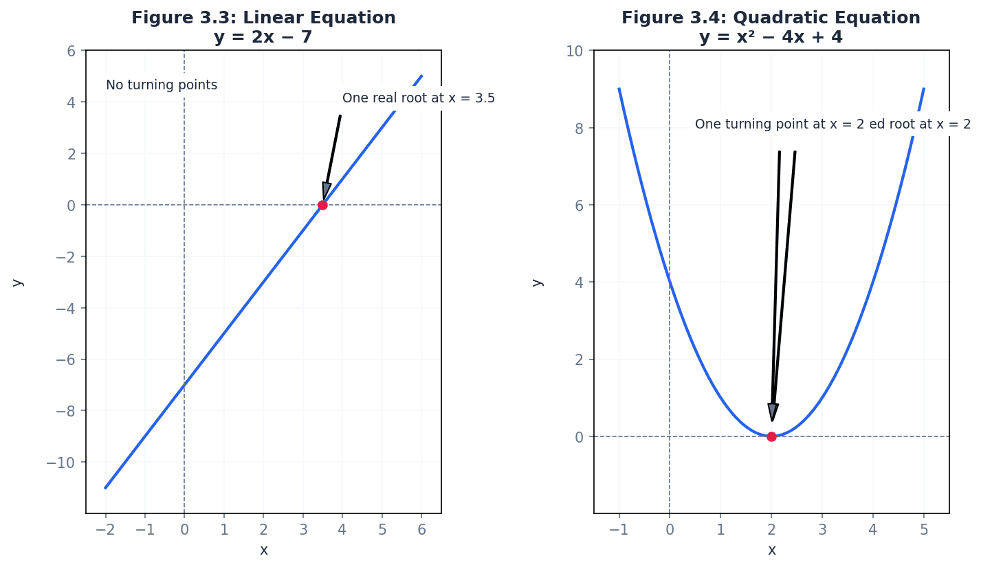
Turning points — The graph of a polynomial function of order n has at most n – 1 turning points.
Turning points are points on the graph where the function changes from increasing to decreasing or vice versa, corresponding to local maxima or minima. The number of turning points is always less than the order of the polynomial. Turning points are like the 'peaks and valleys' on a mountain range; they indicate where the terrain changes direction.
Students often assume a polynomial of order n always has exactly n-1 turning points, but actually it has at most n-1 turning points, and can have fewer (e.g., a cubic with a point of inflection).
Repeated root — A repeated root occurs when two or more distinct roots coincide to become one.
When a root is repeated, the graph of the polynomial touches the x-axis at that point rather than crossing it. This indicates that the factor corresponding to that root appears multiple times in the polynomial's factorization. A repeated root is like two cars arriving at the same destination at the exact same time; they are distinct entities but occupy the same 'space' (value).
Students often overlook repeated roots, counting them as a single root, but actually a repeated root still contributes to the total count of n roots for a polynomial of order n.
Point of inflection — A point of inflection occurs when two turning points of a curve coincide.
At a point of inflection, the concavity of the curve changes (from concave up to concave down or vice versa), but the gradient does not necessarily change sign. For cubic equations, this can mean only one real root. A point of inflection is like a 'twist' in a road where the curve changes direction without necessarily going uphill or downhill.
Students often confuse a point of inflection with a turning point, but actually at a point of inflection the gradient does not change sign (it might be zero, but it doesn't go from positive to negative or vice versa).
An important property of polynomial equations with real coefficients is that their complex roots always occur in conjugate pairs. This means if (a + bi) is a root, then (a - bi) must also be a root. This understanding is crucial when solving equations or determining the nature of roots.
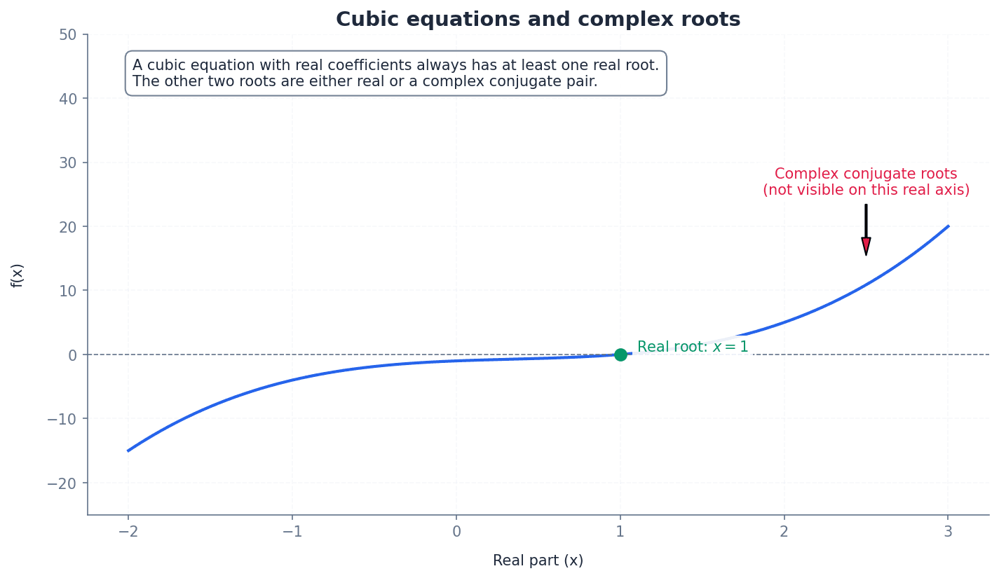
Students often assume all cubic equations have three distinct real roots, but actually they can have one real root and two complex roots, or a repeated real root.
Vieta's formulae establish fundamental relationships between the roots of a polynomial equation and its coefficients. These relationships allow us to find sums and products of roots without explicitly solving the equation, which is particularly useful for quadratic, cubic, and quartic equations. These formulae are essential for evaluating symmetric functions of roots and forming new equations.
Sum of roots for quadratic equation
For a quadratic equation az² + bz + c = 0
Product of roots for quadratic equation
For a quadratic equation az² + bz + c = 0
Sum of roots for cubic equation
For a cubic equation az³ + bz² + cz + d = 0
Sum of products of pairs of roots for cubic equation
For a cubic equation az³ + bz² + cz + d = 0
Product of roots for cubic equation
For a cubic equation az³ + bz² + cz + d = 0
Sum of roots for quartic equation
For a quartic equation az⁴ + bz³ + cz² + dz + e = 0
Sum of products of pairs of roots for quartic equation
For a quartic equation az⁴ + bz³ + cz² + dz + e = 0
Sum of products of triples of roots for quartic equation
For a quartic equation az⁴ + bz³ + cz² + dz + e = 0
Product of roots for quartic equation
For a quartic equation az⁴ + bz³ + cz² + dz + e = 0
Symmetric functions of the roots — Symmetric functions of the roots are functions that remain the same when any two roots are interchanged.
These functions, such as the sum of roots or the sum of products of pairs of roots, can be expressed in terms of the coefficients of the polynomial. This property is crucial for forming new equations or evaluating expressions without explicitly finding the roots. Symmetric functions are like a perfectly balanced seesaw; no matter which two children (roots) swap places, the balance (function value) remains the same.
Symmetric functions of roots can be evaluated directly using Vieta's formulae without needing to find the individual roots. This often involves expressing the desired symmetric function in terms of the elementary symmetric polynomials (e.g., Σα, Σαβ, Σαβγ) and then substituting the values derived from the polynomial's coefficients. This method is generally more efficient and less prone to error than calculating individual roots first.
Students often try to evaluate symmetric functions by finding individual roots first, but actually they can be expressed directly in terms of the polynomial coefficients, which is often more efficient.
When asked to evaluate symmetric functions, always try to express them in terms of Σα, Σαβ, etc., before attempting to find the individual roots, as this is the expected method.
New polynomial equations can be formed whose roots are related to the roots of a given equation, often by a linear transformation. The substitution method is a powerful technique for this. By defining a new variable (e.g., w) in terms of the old variable (z) and the transformation, one can substitute this relationship back into the original equation and simplify to obtain the new polynomial equation in terms of w.
When forming new equations, explicitly state your substitution (e.g., y = x + k) to demonstrate understanding.
Always state Vieta's formulas clearly before applying them to avoid algebraic errors and show your method.
Double-check your calculations, especially when dealing with multiple sums and products for cubic and quartic equations.
Exam Technique
Finding a quadratic equation from given roots
Finding a new equation with roots related by a linear transformation
| Mistake | Fix |
|---|---|
| Confusing expressions with negative or fractional powers as polynomials. | Remember that polynomials must only have positive integer powers of a variable. |
| Confusing the order/degree of a polynomial with the number of terms. | The order/degree is specifically the highest power of the variable, not the count of terms. |
| Assuming all cubic equations have three distinct real roots. | Always consider the possibility of complex roots (which occur in conjugate pairs for real coefficients) or repeated real roots. |
This chapter provides a systematic approach to sketching graphs of rational functions, which are ratios of polynomials. It covers identifying key features like intercepts, various types of asymptotes, and stationary points. Furthermore, it details how to determine the range of these functions and transform their graphs to sketch related functions.
rational number — A number that can be expressed as p/q where p and q are integers and q ≠ 0.
This definition forms the basis for rational functions, extending the concept of a ratio to algebraic expressions. It highlights the fundamental restriction that the denominator cannot be zero, much like a fraction such as 1/2 or 3/4.
rational function — A function that can be expressed in the form y = f(x)/g(x), where f(x) and g(x) are polynomials, and g(x) ≠ 0.
This is the core concept of the chapter, defining the type of functions being studied. The condition g(x) ≠ 0 is crucial as it leads to vertical asymptotes where g(x) = 0. Think of it as an algebraic fraction, where the numerator and denominator are not just numbers, but expressions involving x.
Rational function definition
g(x) ≠ 0; f(x) and g(x) are polynomials of degree 2 or less in this chapter.
Students often think that any function with x in the denominator is rational, but actually both the numerator and denominator must be polynomials.
asymptote — A straight line that a curve approaches tangentially as x and/or y tends to infinity.
Asymptotes are key features of rational function graphs, indicating the behaviour of the function at extreme values of x or y. They are crucial for accurate sketching. Imagine a car driving on a long, straight road that gradually gets closer and closer to a fence without ever touching it; the fence is the asymptote.
Always show asymptotes as dashed lines on your sketches and label them with their equations to gain full marks.
vertical asymptote — A vertical line x = a where the function y = f(x)/g(x) is undefined because g(a) = 0.
These occur at x-values where the denominator of a rational function is zero, causing y to tend to positive or negative infinity. They are found by setting the denominator to zero. It's like a 'wall' that the graph gets infinitely close to but can never touch, because division by zero is impossible.
Students often think that any value of x that makes the denominator zero is a vertical asymptote, but actually if the numerator is also zero at that point, it might be a 'hole' in the graph instead.
To determine the behaviour of the graph near a vertical asymptote, test values of x slightly less than and slightly greater than the asymptote value to see if y tends to +∞ or -∞.
horizontal asymptote — A horizontal line y = c that the curve approaches as x tends to positive or negative infinity.
These describe the end behaviour of the function. They are found by examining the limit of y as x approaches ±∞, often by comparing the degrees of the numerator and denominator polynomials. This is the 'horizon' that the graph approaches as you look far to the left or right, indicating where the y-values settle.
Students often think a horizontal asymptote is always y=0, but actually it can be any constant y=c, or even non-existent if there's an oblique asymptote.
oblique asymptote — A sloping line y = ax + b that a rational function approaches when the degree of the numerator is one greater than that of the denominator.
These asymptotes occur when the function behaves like a linear function for large x. They are found by performing polynomial long division of the numerator by the denominator. Instead of approaching a flat horizon, the graph approaches a sloping 'ramp' as x gets very large.
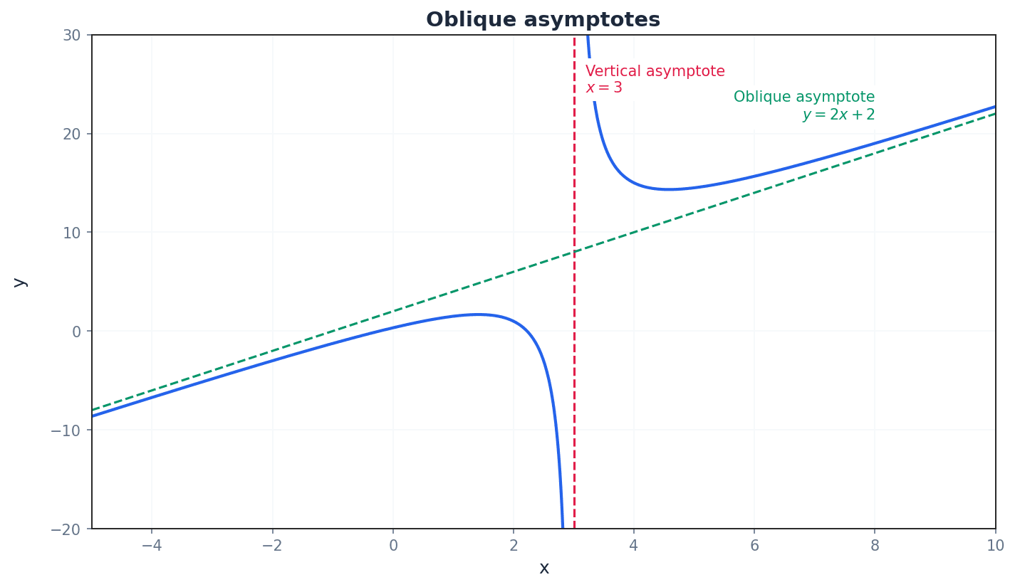
Use polynomial long division to find the equation of an oblique asymptote; the quotient part of the division gives the equation y = ax + b.
Students often confuse the conditions for vertical, horizontal, and oblique asymptotes, especially when comparing the degrees of the numerator and denominator.
Students may incorrectly assume a curve can never cross a horizontal or oblique asymptote. Remember, a curve can cross a horizontal or oblique asymptote, just not a vertical one.
Sketching the graph of a rational function involves a systematic five-step method. This includes finding intercepts by setting x=0 for the y-intercept and y=0 for x-intercepts. Asymptotes (vertical, horizontal, and oblique) are crucial features to identify, along with stationary points where the gradient is zero. Examining the behaviour of the curve near asymptotes and using symmetry properties helps complete an accurate sketch.

stationary point — A point on a curve where the gradient is zero, i.e., dy/dx = 0.
These points correspond to local maxima, local minima, or points of inflection. Finding them is crucial for accurately sketching the shape of the curve and determining its range. Imagine a ball rolling on a hill; a stationary point is where the ball momentarily stops at the very top (maximum) or bottom (minimum) of a dip.
Always calculate the x-coordinates of stationary points by setting dy/dx = 0, and then substitute these back into the original function to find the corresponding y-coordinates.
range — The set of all possible y-values that a function can take.
Understanding the range is essential for fully characterising a function's behaviour. It can be determined from the sketch, by using differentiation to find turning points, or by using the discriminant method. If the domain is all the ingredients you can put into a recipe, the range is all the possible dishes you can make.
Students often think the range is simply all real numbers unless there's an obvious asymptote, but actually stationary points and the overall shape of the graph can restrict the range significantly.
When finding the range, consider the values of y at stationary points and the behaviour of the function as x approaches asymptotes. The discriminant method is a powerful alternative to differentiation for rational functions.
even function — A function f(x) for which f(x) = f(-x), meaning its graph is symmetrical about the y-axis.
Recognising even functions simplifies sketching as only one side of the y-axis needs to be drawn, and the other can be reflected. This saves time and reduces potential errors. It's like folding a piece of paper along the y-axis; the two halves of the graph would perfectly overlap.
Always explicitly state 'f(x) = f(-x)' to prove a function is even, rather than just stating it's symmetrical about the y-axis.
odd function — A function f(x) for which f(x) = -f(-x), meaning its graph has rotational symmetry of order 2 about the origin.
Like even functions, identifying odd functions aids in sketching by allowing reflection about the origin. This property is less common but equally useful when present. If you rotate the graph 180 degrees around the origin, it looks exactly the same.
Always explicitly state 'f(x) = -f(-x)' to prove a function is odd, rather than just stating it has rotational symmetry about the origin.
Understanding how to transform a base graph y = f(x) into related functions like y = |f(x)|, y = f(|x|), y = 1/f(x), and y^2 = f(x) is crucial. Each transformation has specific rules for how it affects the original graph's features, including intercepts, asymptotes, and stationary points. These transformations allow for efficient sketching of complex functions based on simpler ones.
modulus — The absolute numerical value of a number or expression, always taking a positive value.
The modulus function, denoted |f(x)|, transforms any negative y-values of f(x) into their positive counterparts, effectively reflecting parts of the graph below the x-axis. It's like a 'positive-only' filter; whatever number you put in, you only get its positive version out.
Students frequently confuse the transformations y = |f(x)| and y = f(|x|), leading to incorrect reflections. Remember, |f(x)| reflects parts of the graph below the x-axis, while f(|x|) reflects the x>0 part across the y-axis.
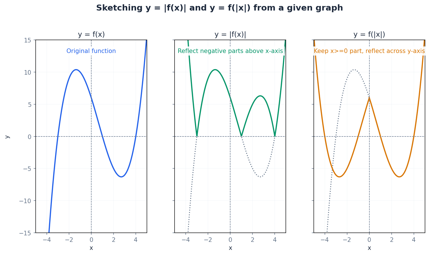
When sketching y = |f(x)|, draw y = f(x) first, then reflect only the portions of the curve where y < 0 in the x-axis. For y = f(|x|), draw y = f(x) for x ≥ 0 and then reflect this part in the y-axis.
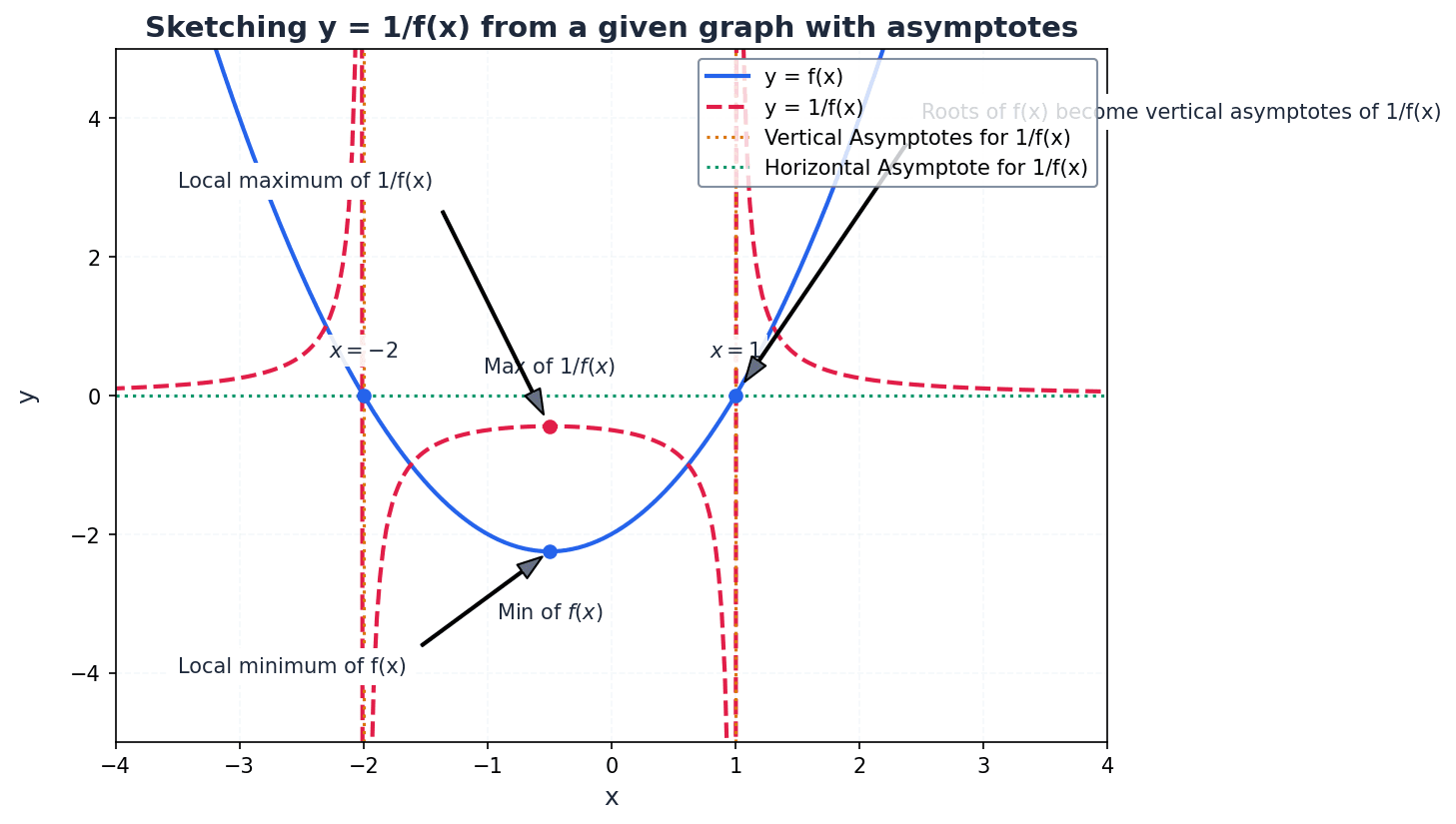
When sketching y = 1/f(x) from y = f(x), several key transformations occur. Roots of f(x) become vertical asymptotes for 1/f(x). Horizontal asymptotes of f(x) at y=c become horizontal asymptotes at y=1/c for 1/f(x). Vertical asymptotes of f(x) become discontinuities (holes) on the x-axis for 1/f(x). Maxima and minima of f(x) become minima and maxima, respectively, for 1/f(x) at the same x-coordinates.
Derivative of 1/f(x)
Used to find stationary points of reciprocal functions and understand how their gradient relates to the original function's gradient.
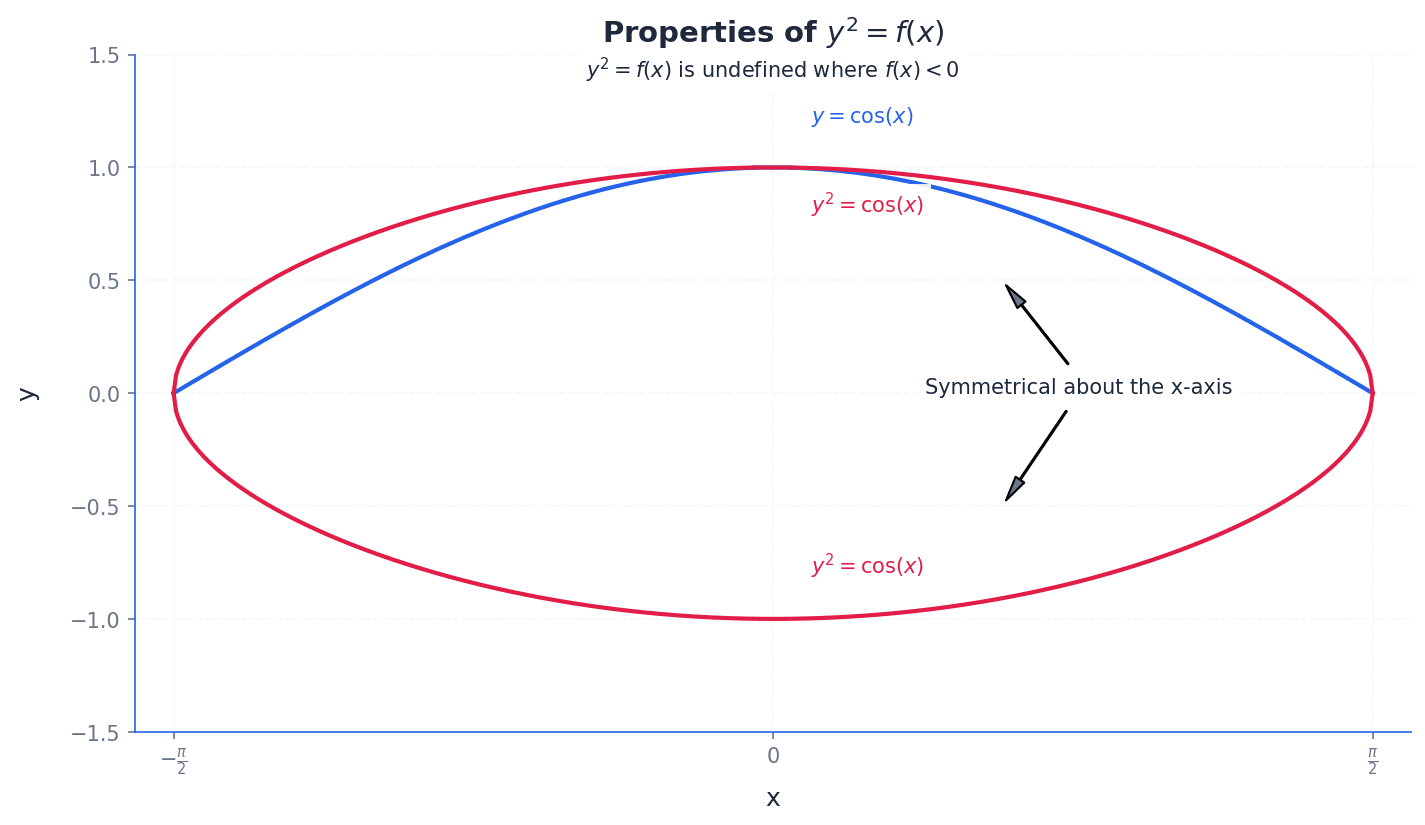
For the transformation y^2 = f(x), the curve is only defined where f(x) ≥ 0, meaning any parts of the original graph below the x-axis are removed. The resulting graph is symmetrical about the x-axis. x-intercepts of f(x) remain x-intercepts for y^2 = f(x), and the curve passes vertically through them. Maximum points (x,y) on f(x) become (x, ±√ y) on y^2 = f(x).
Students may forget that y^2 = f(x) is only defined where f(x) ≥ 0, leading to sketching parts of the curve that do not exist.
When sketching, always clearly label all asymptotes, intercepts (x and y), and stationary points.
For range questions, be prepared to use either differentiation (finding turning points) or the discriminant (rearranging to a quadratic in x).
When transforming graphs, systematically apply the rules for y = |f(x)|, y = f(|x|), y = 1/f(x), and y^2 = f(x) to key features.
Exam Technique
Sketching the graph of a rational function y = f(x)/g(x)
Determining the range of a rational function
| Mistake | Fix |
|---|---|
| Confusing the conditions for vertical, horizontal, and oblique asymptotes. | Carefully compare the degrees of the numerator and denominator polynomials. Vertical: denominator = 0. Horizontal: degree(num) ≤ degree(den). Oblique: degree(num) = degree(den) + 1. |
| Assuming a curve can never cross a horizontal or oblique asymptote. | Remember that a curve can cross horizontal or oblique asymptotes for finite x-values; it only approaches them as x tends to infinity. It cannot cross vertical asymptotes. |
| Forgetting to check the behaviour of y (tending to +∞ or -∞) on both sides of a vertical asymptote. | Always test x-values slightly to the left and right of each vertical asymptote to determine the direction of the curve. |
This chapter introduces polar coordinates (r, θ) as an alternative to Cartesian coordinates (x, y) for describing points in a plane. It covers the conversion between these two coordinate systems for both points and equations of curves, and details how to sketch simple polar curves and calculate the area they enclose using integration.
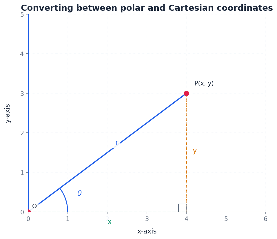
polar coordinates — The numbers (r, θ) that describe the position of a point P by its distance r from a fixed point O (the pole) and the angle θ between OP and an initial line.
Polar coordinates offer an alternative to Cartesian coordinates, particularly useful for curves with rotational symmetry. The distance r is always non-negative, and the angle θ is typically measured in radians anticlockwise from the initial line. Imagine a radar screen: 'r' is how far away a target is from the center, and 'θ' is its bearing (direction) from a fixed reference line.
pole — A fixed point O from which the distance r to a point P is measured in polar coordinates.
The pole serves as the origin in the polar coordinate system, analogous to the origin (0,0) in Cartesian coordinates. At the pole, r=0 and θ is undefined. The pole is like the bullseye of a dartboard; all distances are measured outwards from it.
initial line — A line drawn horizontally to the right from the pole, used as the reference for measuring the angle θ in polar coordinates.
The initial line is the angular reference (θ=0) in the polar system, similar to the positive x-axis in Cartesian coordinates. Angles are typically measured anticlockwise from this line. Think of the initial line as the starting point on a protractor, from which you measure angles.
principal polar coordinates — A unique set of polar coordinates (r, θ) for a point where r > 0 and −π < θ < π.
These coordinates provide a unique representation for each point in the plane, resolving the issue of infinite possible (r, θ) pairs for a single point. This convention is similar to the modulus-argument form for complex numbers. If polar coordinates are like having many nicknames, principal polar coordinates are like having one official name that everyone uses.
Students often think that each point has a unique set of polar coordinates (r, θ), but actually adding or subtracting any integer multiple of 2π to θ defines the same point. Remember that principal polar coordinates are specifically defined to ensure uniqueness.
When asked to define a point using polar coordinates, be aware that multiple (r, θ) pairs can represent the same point unless principal polar coordinates are specified. When asked for 'the polar coordinates' of a point, providing the principal polar coordinates is usually expected for a unique answer.
r — The distance of a point P from the pole O in polar coordinates.
r is the radial distance and is always considered non-negative in the standard convention. It forms the hypotenuse of a right-angled triangle when converting to Cartesian coordinates. r is like the radius of a circle that passes through the point P, centered at the pole.
θ — The angle between the line segment OP and the initial line in polar coordinates.
θ is typically measured in radians, in an anticlockwise direction from the initial line. It determines the angular position of the point P. θ is like the hand on a clock, but instead of hours, it measures the angle from a fixed starting point.
x — The Cartesian coordinate representing the horizontal distance from the y-axis.
In the conversion between polar and Cartesian systems, x is related to r and θ by x = r cosθ. It is the horizontal component of the point's position. If you walk 'r' steps at an angle 'θ', 'x' is how far you've moved horizontally from your starting point.
y — The Cartesian coordinate representing the vertical distance from the x-axis.
In the conversion between polar and Cartesian systems, y is related to r and θ by y = r sinθ. It is the vertical component of the point's position. If you walk 'r' steps at an angle 'θ', 'y' is how far you've moved vertically from your starting point.
Understanding the relations between Cartesian and polar coordinates is fundamental. Points and equations can be converted between these two systems. The conversion formulas are derived from basic trigonometry, relating the radial distance 'r' and angle 'θ' to the horizontal 'x' and vertical 'y' components.
Cartesian x-coordinate from polar
Used to convert from polar to Cartesian coordinates.
Cartesian y-coordinate from polar
Used to convert from polar to Cartesian coordinates.
Polar r-coordinate from Cartesian
Used to convert from Cartesian to polar coordinates. r is always positive.
Polar θ-coordinate from Cartesian
Used to convert from Cartesian to polar coordinates. Care must be taken to choose the right quadrant for θ.
When finding θ from Cartesian coordinates, always draw a sketch to ensure you choose the correct quadrant, as tan(θ) gives two possible values. This helps avoid errors when converting points like (√3, 1) to polar form.
When converting from Cartesian to polar coordinates, students may choose the wrong quadrant for θ if they only rely on tanθ = y/x without drawing a sketch.
Sketching simple polar curves involves understanding how r varies with θ. Key features to identify include intersections with the initial line (θ=0, π), and the greatest and least values of r. Curves like the Rhodonea (rose curve), Spiral of Archimedes, Cardioid, and Lemniscate are common examples.
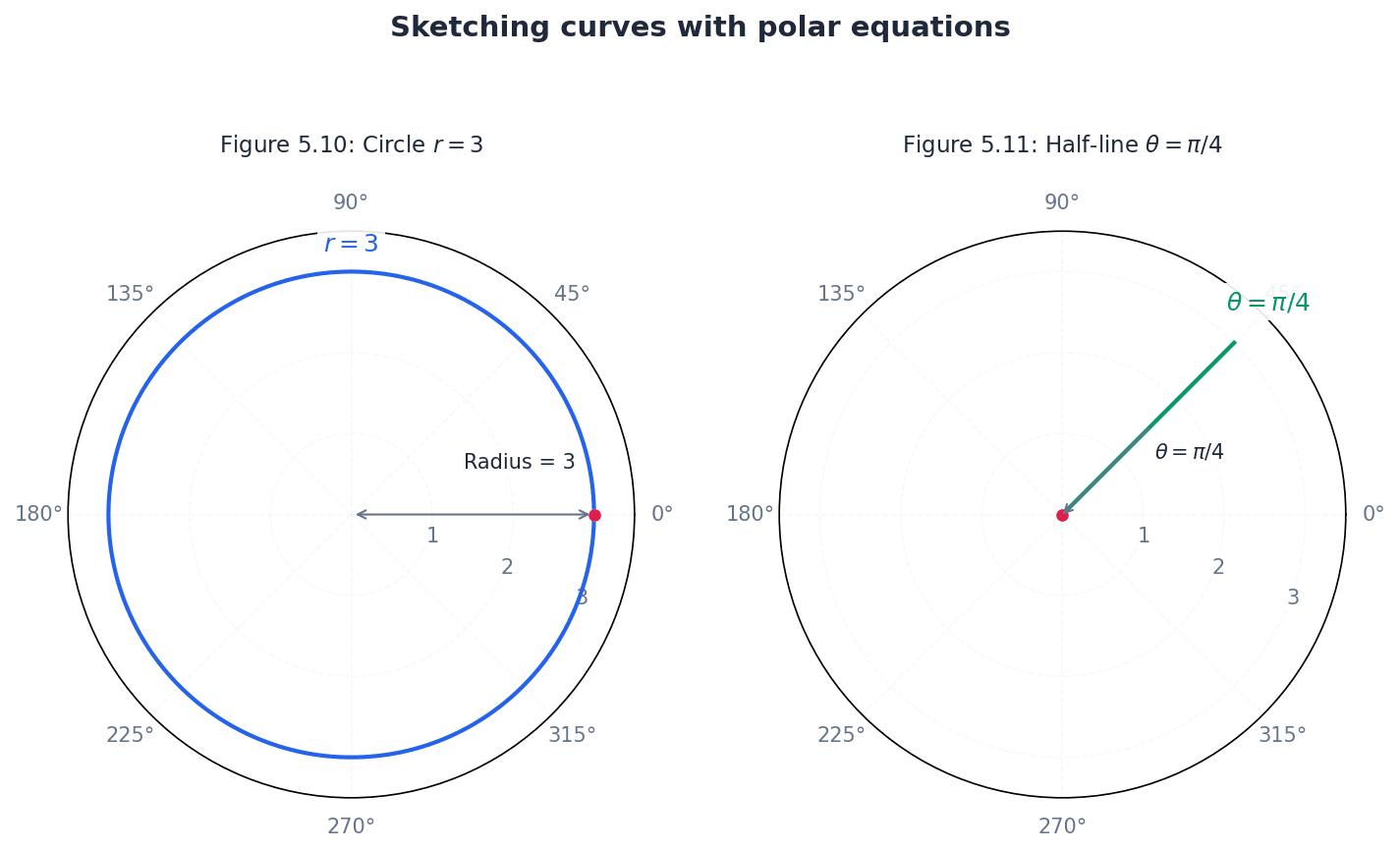
Always draw the initial line correctly when sketching polar curves, as it defines the orientation of the graph and affects how angles are interpreted. When sketching polar curves, pay close attention to the range of θ for which r is positive, as negative r values are typically excluded in this course.
Students might incorrectly assume r can be negative when sketching curves, but in this course, the convention is to only consider positive values of r. Also, do not confuse the graph of θ = constant (a half-line) with y = x (a full line through the origin).
Determining the symmetry of polar curves can greatly simplify sketching. Symmetry about the initial line (θ=0) can be tested by replacing θ with -θ. Symmetry about the line θ=π/2 can be tested by replacing θ with π-θ. Symmetry about the pole can be tested by replacing r with -r.
To find the greatest and least values of r for a polar curve, analyze the function r(θ). For trigonometric functions, this often involves finding the maximum and minimum values of the cosine or sine terms. These extreme values correspond to the points furthest from and closest to the pole, respectively.
The area enclosed by a polar curve is calculated using integration. The formula for the area of a sector in polar coordinates is derived from considering infinitesimal triangular elements. This method allows for finding the area of regions bounded by a polar curve and two radial lines.
Area enclosed by a polar curve
Used to find the area of a region bounded by a polar curve and two straight lines θ=α and θ=β.
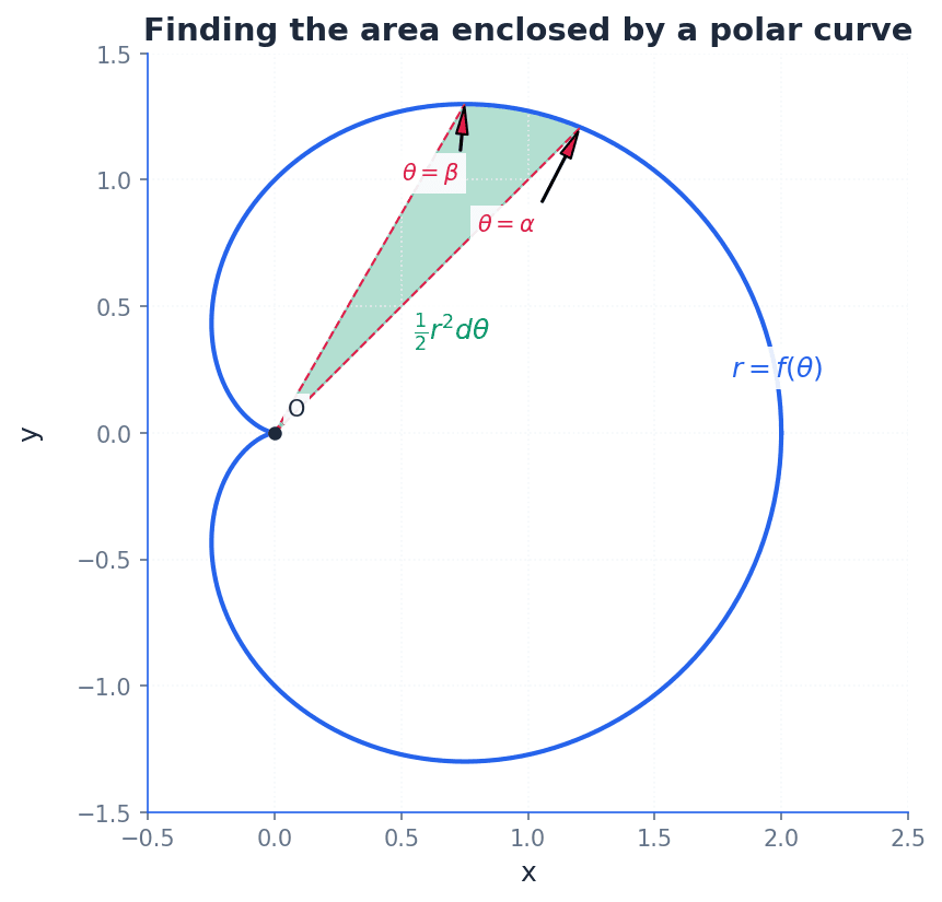
When finding the area enclosed by a polar curve, students might use incorrect limits of integration or forget to square r in the formula A = (1/2) ∫ r² dθ.
For area calculations, carefully determine the correct limits of integration (α and β) for the specific region required. Remember to expand r^2 and use trigonometric identities like cos^2θ = (1/2)(1 + cos2θ) to simplify the integrand before integration.
When sketching polar curves, identify significant features like intersections with the initial line (θ=0, π) and greatest/least values of r. To find greatest/least values of r, differentiate r with respect to θ and set dr/dθ = 0, or analyse trigonometric functions.
Always sketch the point or curve when converting coordinates or equations to avoid quadrant errors for θ. This visual aid is crucial for accuracy in polar coordinates.
Exam Technique
Convert Cartesian coordinates (x, y) to polar coordinates (r, θ)
Convert polar coordinates (r, θ) to Cartesian coordinates (x, y)
| Mistake | Fix |
|---|---|
| Assuming each point has a unique set of polar coordinates. | Remember that (r, θ) and (r, θ + 2nπ) represent the same point. Use principal polar coordinates (r > 0, -π < θ < π) for a unique representation unless otherwise specified. |
| Choosing the wrong quadrant for θ when converting from Cartesian to polar coordinates. | Always draw a sketch of the Cartesian point (x, y) to visually determine the correct quadrant for θ, as tanθ = y/x gives two possible angles. |
| Assuming r can be negative when sketching polar curves. | In this course's convention, r is taken to exist only for positive values. If your equation yields negative r, you should typically omit these points or understand the specific convention being used (e.g., plotting in the opposite direction). |
This chapter introduces matrices and their inverses, focusing on 2x2 and 3x3 matrices. It defines the determinant as an area or volume scale factor for transformations and explains its significance, particularly for singular matrices. The chapter covers methods for finding the inverse of non-singular matrices, including the adjugate method for 3x3 matrices, and properties of inverses for matrix products.
determinant — The quantity (ad − bc) is the area scale factor associated with the transformation matrix.
For a 2x2 matrix, the determinant indicates how much the area of a shape is scaled by the transformation. A negative determinant signifies a reversal in the order of vertices, like flipping a rubber sheet over. For a 3x3 matrix, it represents the volume scale factor.
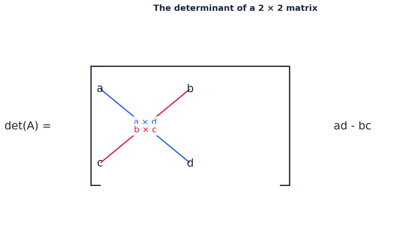
Determinant of a 2 × 2 matrix
Represents the area scale factor of the transformation. If negative, indicates a reversal of orientation.
Students often confuse a negative determinant with a negative area. Remember that area cannot be negative; the negative sign indicates a reversal in the orientation of the transformed shape.
When asked to find the area of a transformed shape, remember to use the absolute value of the determinant as the area scale factor. For 3x3 matrices, the determinant is the volume scale factor.
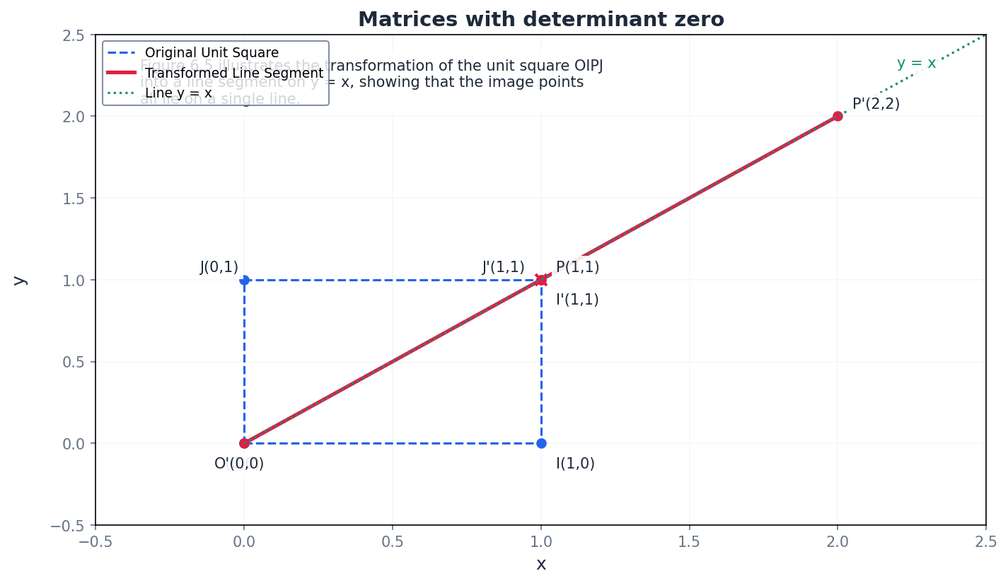
singular — If the determinant of a matrix is zero then the inverse matrix does not exist and the matrix is said to be singular.
A singular matrix maps all points on the plane to a straight line (in 2D) or to a plane (in 3D), meaning an infinite number of points map to the same image point. This makes it impossible to uniquely reverse the transformation, hence no inverse exists. It's like trying to reverse a process where many different starting points lead to the exact same outcome.
non-singular — If det M ≠ 0 the matrix is said to be non-singular.
A non-singular matrix has a non-zero determinant, which means its inverse exists. This type of matrix represents a transformation that can be uniquely reversed, as it does not collapse dimensions. It's like a reversible operation, such as stretching a rubber band; you can always stretch it back to its original state.
If a question asks for values that make a matrix singular, set the determinant equal to zero and solve for the unknown variable. This is a common way to test understanding of the term.
identity matrix — The matrix \begin{pmatrix} 1 & 0 \\ 0 & 1 \end{pmatrix} is known as the 2 × 2 identity matrix, which maps every point to itself.
Identity matrices, denoted by I, behave like the number 1 in real number multiplication; when multiplied by any matrix M, the product is M. This matrix represents a transformation that leaves all points unchanged, like doing nothing at all to a shape.
Students often think the identity matrix is always \begin{pmatrix} 1 & 1 \\ 1 & 1 \end{pmatrix}. Remember that it has 1s on the main diagonal and 0s elsewhere, ensuring it acts as a multiplicative identity.
inverse — If the product of two square matrices, M and N, is the identity matrix I, then N is the inverse of M, written as N = M−1.
The inverse matrix 'undoes' the transformation represented by the original matrix. If a transformation A maps P to Q, then A−1 maps Q back to P. An inverse only exists for non-singular matrices. It's like a set of instructions to move an object back to its original position after it has been moved.
Students often think all matrices have an inverse. Remember that only non-singular matrices (those with a non-zero determinant) have an inverse.
Inverse of a 2 × 2 matrix
Exists only if det M = (ad - bc) ≠ 0 (i.e., M is non-singular).
When finding an inverse, always calculate the determinant first. If it's zero, state that the inverse does not exist and the matrix is singular, as this earns marks.
The determinant of a 3x3 matrix represents the volume scale factor of the transformation it describes. It can be found by expanding along any row or column, using a pattern of minors and cofactors. For example, expanding by the first column involves multiplying each element by its corresponding cofactor and summing the results.
Determinant of a 3 × 3 matrix (expansion by first column)
Represents the volume scale factor of the transformation. Can also be expanded by other columns or rows using the cofactor sign pattern.
minor — The 2 × 2 determinant obtained by deleting the row and column containing an element is called the minor of that element.
For a 3x3 matrix, each element has a corresponding minor. These minors are crucial intermediate steps in calculating the determinant and the cofactors, which are then used to find the inverse matrix. Think of a minor as a 'sub-determinant' or a smaller puzzle piece within the larger matrix puzzle.
cofactor — A minor, together with its correct sign, is known as a cofactor and is denoted by the corresponding capital letter.
The sign of a cofactor depends on its position in the matrix, following an alternating pattern (+ - + / - + - / + - +). Cofactors are used in the expansion of the determinant and in forming the adjugate matrix for finding the inverse. If a minor is the raw value, the cofactor is that value with a 'directional' sign attached.
Students often confuse minors with cofactors. Remember that a minor is just the determinant of the sub-matrix, while a cofactor includes the correct sign based on its position.
Always remember the sign pattern for cofactors: + − + / − + − / + − +. A single sign error will propagate through the entire calculation for the determinant or inverse, resulting in loss of marks.
adjugate — The matrix formed by replacing each element of M by its cofactor and then transposing the matrix (i.e. changing rows into columns and columns into rows) is known as the adjugate or adjoint of M, denoted adj M.
The adjugate matrix is a key component in the formula for finding the inverse of a 3x3 matrix. It is derived from the matrix of cofactors, which is then transposed. If the cofactors are individual pieces of a puzzle, the adjugate matrix is like arranging those pieces into a new, specific pattern (transposed) that, when combined with the determinant, reveals the inverse.
Inverse of a 3 × 3 matrix
Exists only if det M ≠ 0. The adjugate matrix is the transpose of the matrix of cofactors.
Students often forget to transpose the matrix of cofactors to get the adjugate. Remember that this transposition step is essential for the formula for the inverse.
Ensure you correctly calculate all cofactors and then transpose the matrix of cofactors. A common mistake is to transpose before calculating all cofactors or to forget the transposition entirely.
When dealing with the product of two non-singular matrices, the inverse of their product follows a specific rule. The inverse of a product (AB) is the product of their individual inverses, but in reverse order, i.e., B⁻¹A⁻¹. This property can be extended to the product of more than two matrices.
Inverse of a product of matrices
Applies to non-singular matrices M and N of the same order. The order of inversion is reversed.
Students often incorrectly apply the order of inversion for matrix products. Remember it is (MN)⁻¹ = N⁻¹M⁻¹, not M⁻¹N⁻¹.
For 3x3 inverses, clearly show the calculation of minors, cofactors, and the adjugate matrix to gain full method marks.
Utilise your calculator for finding the inverse of 3x3 matrices to check your manual calculations, but be prepared to show full working if required.
Exam Technique
Find the determinant of a 2x2 matrix
Find the inverse of a 2x2 matrix
| Mistake | Fix |
|---|---|
| Confusing a negative determinant with a negative area. | Remember that area cannot be negative; the negative sign indicates a reversal in the orientation of the transformed shape. |
| Assuming all matrices have an inverse. | Only non-singular matrices (those with a non-zero determinant) have an inverse. Always check the determinant first. |
| Mistaking minors for cofactors. | A minor is the determinant of the sub-matrix. A cofactor is the minor with the correct alternating sign applied based on its position. |
This chapter extends vector concepts to three-dimensional geometry, focusing on planes and their interactions with lines. It covers various forms of plane equations, methods for finding them, and how to determine intersections, angles, and shortest distances between lines and planes, and between two planes. A key new concept is the vector product, essential for finding normal vectors and distances between skew lines.
magnitude — The length or size of a vector.
Magnitude is a scalar quantity that describes the extent of a vector, such as the speed of an object or the strength of a force. If a vector is an arrow, its magnitude is the length of the arrow.
direction — The orientation of a vector in space.
Direction specifies where a vector is pointing, often given by angles relative to coordinate axes or as a unit vector. If a vector is an arrow, its direction is where the arrow is pointing.
position vector — A vector that represents the position of a point in space relative to an origin.
A position vector starts at the origin and ends at the point, uniquely defining the point's location. Think of a position vector as the GPS coordinates for a specific location, but expressed as a vector from a central starting point.
scalar product — A product of two vectors that results in a scalar quantity, calculated as a · b = |a||b|cosθ.
The scalar product (also known as the dot product) measures the extent to which two vectors point in the same direction and is useful for finding the angle between vectors or checking for perpendicularity. Imagine two people pulling ropes; the scalar product tells you how much of their effort is aligned, contributing to movement in the same direction.
Students often think the scalar product results in a vector, but actually it always produces a single number (a scalar).
Remember that a · b = 0 implies vectors a and b are perpendicular (unless one is a zero vector), a common test in exam questions.
normal to the plane — A line or vector that is perpendicular to every line in a given plane.
The normal vector defines the orientation of the plane in space; its direction is unique (up to a scalar multiple) for any given plane. If a plane is a flat table, the normal vector is like a pencil standing perfectly upright on that table, perpendicular to its surface.
Students often think 'normal' means 'usual', but actually in mathematics, 'normal' means perpendicular or at right angles.
The coefficients of x, y, and z in the Cartesian equation of a plane (ax + by + cz = d) directly give the components of a normal vector to that plane, which is a crucial shortcut.
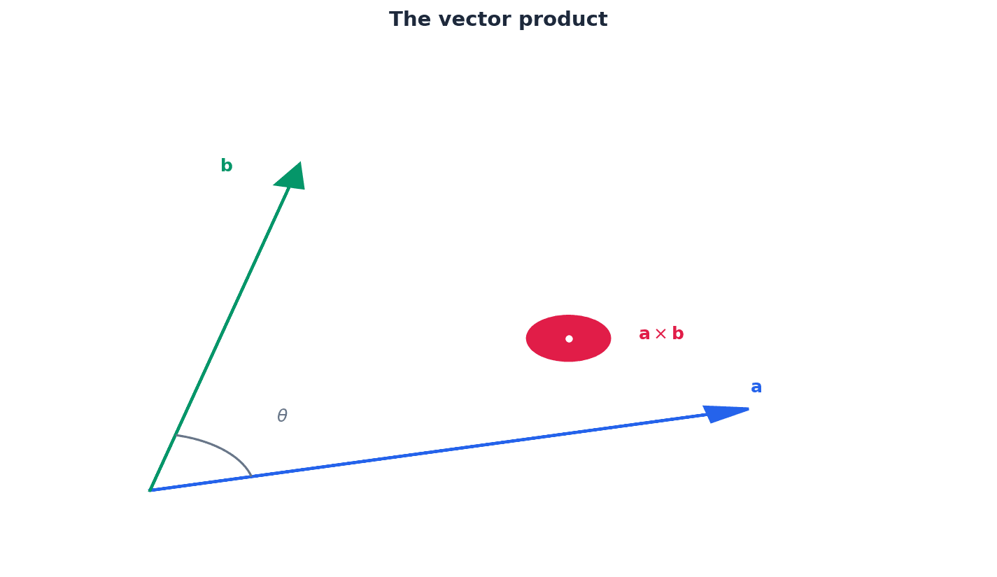
vector product — A product of two vectors that results in a vector perpendicular to both original vectors, calculated as a × b = |a||b|sinθ n̂.
The vector product (also known as the cross product) produces a vector whose magnitude is the area of the parallelogram formed by the two vectors, and whose direction is given by the right-hand rule, perpendicular to the plane containing the two vectors. If you have two vectors representing forces, their vector product can represent a torque, which is a rotational force perpendicular to both original forces.
Students often confuse scalar product (dot product) with vector product (cross product) and their resulting types (scalar vs. vector).
The vector product is essential for finding a normal vector to a plane given two vectors within the plane, and for calculating the area of a triangle or parallelogram.
anti-commutative property — A property of the vector product where a × b = − b × a.
This means that reversing the order of the vectors in a vector product reverses the direction of the resulting vector, while its magnitude remains the same. If turning a screw clockwise drives it in, turning it anti-clockwise drives it out; the action is the same, but the direction is opposite.
Students often think the vector product is commutative (a × b = b × a), but actually it is anti-commutative (a × b = -b × a).
Be careful with the order of vectors in a vector product, as swapping them introduces a negative sign, which can lead to errors in direction-dependent calculations.
sheaf of planes — An arrangement where several planes share a common line of intersection.
When two planes intersect, they form a line; any other plane containing this same line is part of the sheaf, meaning all planes in the sheaf pass through that common line. Think of the pages of an open book; each page is a plane, and the spine of the book is the common line of intersection for all those 'planes'.
Students often think a sheaf of planes means they all intersect at a single point, but actually they all share a common line, not necessarily a single point.
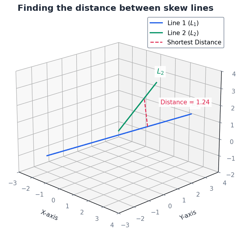
skew lines — Two lines in three dimensions that do not intersect and are not parallel.
Skew lines exist in different planes and never meet, unlike parallel lines (which are in the same plane) or intersecting lines (which meet at a point). Imagine two aeroplanes flying at different altitudes and on different headings; they might pass close to each other but never collide if their paths are skew.
Students often think 'not intersecting' means 'parallel', but actually skew lines are a distinct case where they are neither parallel nor intersecting.
Vector equation of a plane (parametric form)
Used when three points A, B, C on the plane are known. Can also be written as r = a + λ(b − a) + µ(c − a).
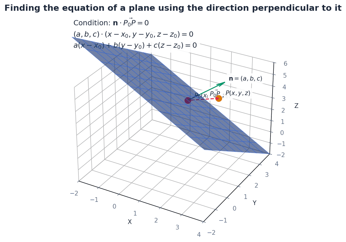
Cartesian equation of a plane
General form of a plane's equation. The vector (a, b, c) is perpendicular to the plane.
Vector equation of a plane (normal form)
Used when a point on the plane and a normal vector to the plane are known. Can be expanded to r · n = a · n.
Planes in three-dimensional space can be represented in various forms. The vector equation of a plane can be expressed parametrically using a position vector of a point on the plane and two non-parallel direction vectors within the plane. Alternatively, the normal form of the vector equation uses a position vector of a point on the plane and a vector perpendicular to the plane, known as the normal vector. These vector forms can be converted into the Cartesian equation of a plane, ax + by + cz = d, where (a, b, c) are the components of the normal vector.
When converting between vector and Cartesian forms, show clear algebraic steps, especially when eliminating parameters.
To find the intersection of a line and a plane, the parametric equations of the line (x, y, z in terms of a parameter) are substituted into the Cartesian equation of the plane. Solving the resulting equation for the parameter yields the specific value at the intersection point. If no solution exists, the line is parallel to the plane; if an identity is formed, the line lies within the plane.
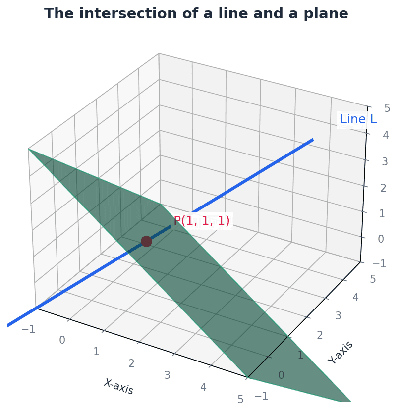
For intersection problems, substitute the line equation into the plane equation and solve for the parameter.
The angle between a line and a plane is determined by considering the line's direction vector and the plane's normal vector. The scalar product of these two vectors can be used to find the angle between them. The angle between the line and the plane itself is then 90 degrees minus this calculated angle, as the normal vector is perpendicular to the plane.
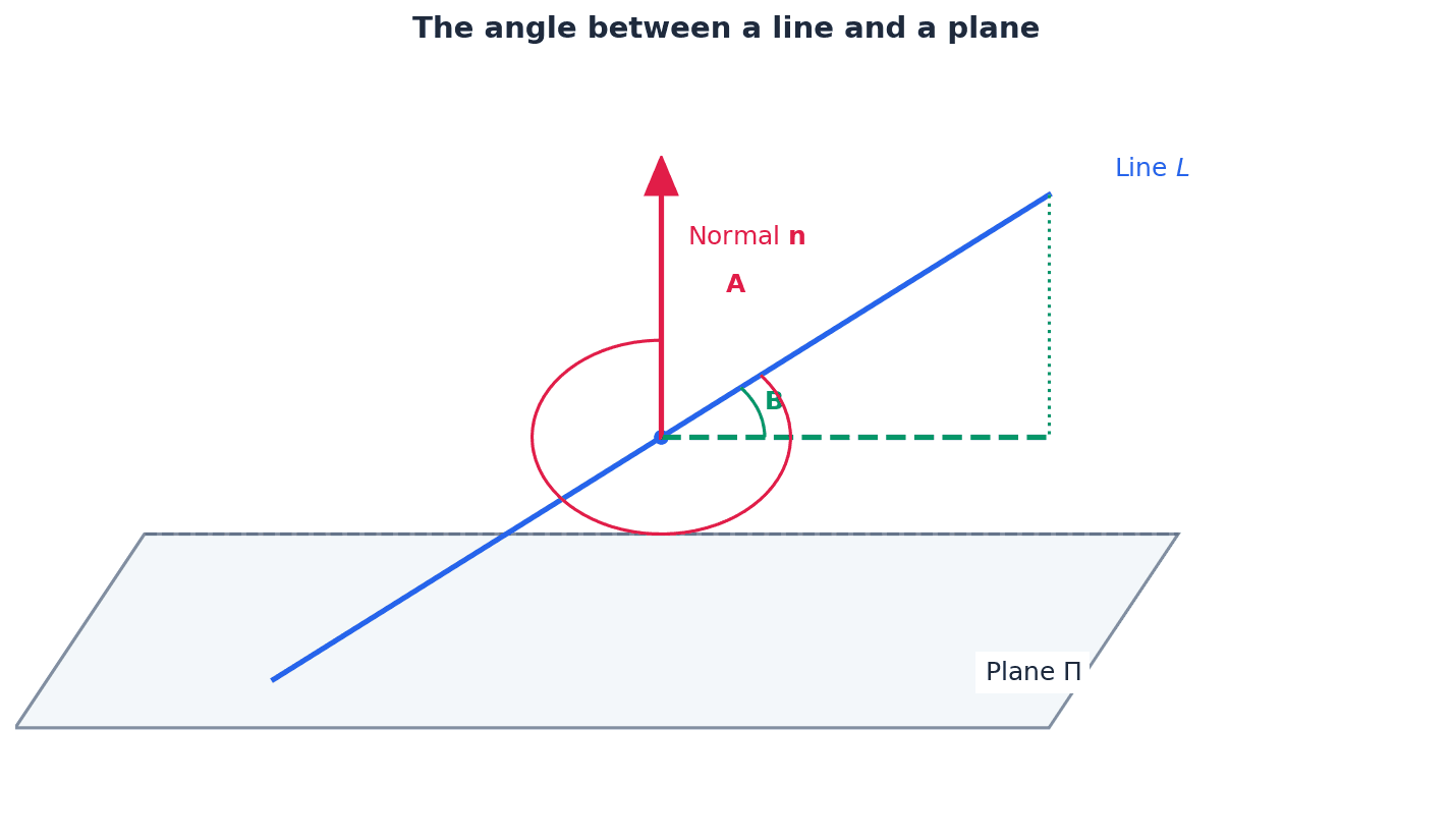
Students often use the wrong angle (e.g., angle with normal instead of angle with plane) when calculating the angle between a line and a plane. Remember to use 90° minus the angle between the line's direction vector and the plane's normal vector.
The vector product, or cross product, of two vectors a and b, denoted a × b, yields a new vector that is perpendicular to both a and b. Its magnitude is given by |a||b|sinθ, representing the area of the parallelogram formed by the two vectors. The direction of the resulting vector is determined by the right-hand rule. A key property is its anti-commutative nature: a × b = -b × a.
Vector product (definition)
Results in a vector perpendicular to both a and b. Magnitude is the area of the parallelogram formed by a and b.
Vector product (component form)
Used for calculating the vector product when vectors are given in component form.
Vector product (determinant form)
An alternative way to express and calculate the vector product using a determinant expansion.
Incorrectly applying the right-hand rule for the direction of the vector product can lead to sign errors.
Calculating shortest distances is a crucial application of vectors. The distance from a point to a plane can be found using a specific formula involving the plane's Cartesian equation and the point's coordinates. For a point to a line in 3D, the vector product is used, involving a vector from a point on the line to the given point, and the line's direction vector. The most complex case is finding the shortest distance between two skew lines, which involves both the scalar and vector products of their direction vectors and a vector connecting points on each line.
Distance of a point from a plane
Provides the shortest perpendicular distance from a given point to a plane.
Distance from a point to a line (3D)
Calculates the shortest perpendicular distance from a point to a line in three dimensions.
Distance from a point to a line (2D)
Calculates the shortest perpendicular distance from a point to a line in two dimensions.
Distance between two skew lines
Calculates the shortest perpendicular distance between two lines that are not parallel and do not intersect.
Forgetting to take the absolute value in distance formulas can lead to negative distances, which are physically impossible.
Practice distance formulas thoroughly, especially for skew lines, as these can be complex and require careful calculation.
Always check your final answers for reasonableness, especially for angles and distances.
Exam Technique
Finding the equation of a plane given three points
Finding the equation of a plane given a point and a normal vector
| Mistake | Fix |
|---|---|
| Confusing scalar product (dot product) with vector product (cross product) and their resulting types (scalar vs. vector). | Remember that the scalar product yields a scalar (a number), while the vector product yields a vector. Pay attention to the notation (· vs ×). |
| Incorrectly applying the right-hand rule for the direction of the vector product, leading to sign errors. | Practice the right-hand rule consistently. Remember that a × b = -b × a (anti-commutative property). |
| Assuming lines are parallel if they don't intersect, rather than checking for skew lines in 3D. | Always check if direction vectors are scalar multiples to determine parallelism. If not parallel and no intersection point exists, the lines are skew. |
Generated by Nexelia Academy · nexeliaacademy.com