Further Pure Mathematics 1 · Matrices and transformations
This chapter introduces matrices as rectangular arrays of numbers, defining their order and special types. It covers fundamental matrix operations and explores how matrices represent 2D geometric transformations. Finally, it discusses successive transformations, invariant points, and invariant lines.
matrix — A matrix is an array of numbers, usually written inside curved brackets.
Matrices are used to represent data or transformations. They consist of rows and columns, with individual entries called elements. Think of a matrix like a spreadsheet or a grid of numbers, where each cell holds a specific value and its position matters.
elements — The entries in the various cells of a matrix are known as elements.
Each number or variable within a matrix is an element. Their position within the matrix (row and column index) is important for matrix operations and defining the matrix's order. If a matrix is a bookshelf, then each book on the shelf is an element.
order — The order of a matrix is stated by the number of rows first, then the number of columns.
For example, a 5 × 5 matrix has five rows and five columns. The order is fundamental as it determines whether matrices can be added, subtracted, or multiplied. The order of a matrix is like the dimensions of a room – length by width.
Always state the order correctly as 'rows × columns'; reversing this will lose marks, especially in questions about conformability.
square matrices — Matrices that have the same number of rows as columns are called square matrices.
Examples include 2 × 2 or 3 × 3 matrices. Square matrices are important for operations like finding determinants, inverses, and representing certain transformations. A square matrix is like a square grid or a chessboard, where the number of rows equals the number of columns.
identity matrix — An identity matrix is a square matrix with 1s on the leading diagonal and zeros elsewhere, usually denoted by I.
When an identity matrix multiplies another matrix, the other matrix remains unchanged, similar to how multiplying a number by 1 leaves it unchanged. Identity matrices must be square. The identity matrix is like the number '1' in scalar multiplication; it leaves the other matrix unchanged when multiplied.
unit matrix — The unit matrix is another name for the identity matrix.
It serves the same purpose as the identity matrix, leaving other matrices unchanged upon multiplication. It is always a square matrix with ones on the main diagonal and zeros elsewhere. Just like a 'unit' of measurement is a standard, the unit matrix is the standard 'multiplicative identity' for matrices.
Remember that I can be of any square order (e.g., I₂ or I₃) and its specific order is usually implied by the context of the multiplication.
zero matrix — A zero matrix is a matrix where all elements are zero, usually denoted by O.
When a zero matrix is added to another matrix, the other matrix remains unchanged, similar to how adding 0 to a number leaves it unchanged. Zero matrices can be of any order. The zero matrix is like the number '0' in scalar addition; it leaves the other matrix unchanged when added.
equal matrices — Two matrices are said to be equal if, and only if, they have the same order and each element in one matrix is equal to the corresponding element in the other matrix.
This means that for matrices A and B to be equal, they must have the same number of rows and columns, and aᵢⱼ must equal bᵢⱼ for all i and j. Two matrices being equal is like having two identical jigsaw puzzles; they must have the same number of pieces (order) and each piece must match its corresponding piece in the other puzzle (elements).
Matrices can be added or subtracted if they have the same order. This involves adding or subtracting corresponding elements. If matrices are not of the same order, they are non-conformable for addition, and the operation is undefined. Scalar multiplication involves multiplying every element within a matrix by a single number, called a scalar, which changes the magnitude of the elements but not the matrix's order.
non-conformable for addition — Matrices are non-conformable for addition if they are not of the same order.
Matrix addition and subtraction require matrices to have identical dimensions (same number of rows and columns) because elements are added or subtracted in corresponding positions. Trying to add non-conformable matrices is like trying to add apples and oranges; they are different types of items and cannot be combined directly.
scalar number — A scalar number is a single number by which a matrix can be multiplied.
When a matrix is multiplied by a scalar, every element within the matrix is multiplied by that scalar. This operation changes the magnitude of the matrix elements but not its order. Multiplying a matrix by a scalar is like scaling a recipe; if you double the recipe (scalar factor of 2), you double every ingredient (element).
Students often think scalar multiplication only applies to certain elements, but actually it applies to every single element in the matrix.
Matrix multiplication is a more complex operation than addition or scalar multiplication. Two matrices are conformable for multiplication if the number of columns in the first matrix equals the number of rows in the second matrix. The resulting product matrix will have an order determined by the outer dimensions of the original matrices. Each element of the product is found by multiplying elements of a row from the first matrix by elements of a column from the second matrix and summing the products.
conformable for multiplication — Two matrices are conformable for multiplication if the number of columns in the first matrix equals the number of rows in the second matrix.
For matrices A (order m × n) and B (order n × p), the product AB exists because the 'middle' numbers (n) are the same. The resulting product matrix will have the order m × p. Being conformable for multiplication is like connecting two gears; the number of teeth on the output of the first gear must match the number of teeth on the input of the second gear for them to mesh.
Matrix Multiplication (2x2)
The product of a 2x2 matrix with another 2x2 matrix results in a 2x2 matrix. Each element of the product is found by multiplying elements of a row from the first matrix by elements of a column from the second matrix and summing the products.
Students often think any two matrices can be multiplied, but actually they must be conformable for multiplication (inner dimensions must match).
Always write down the orders of the matrices (e.g., 2×4 and 4×1) to visually check if the inner numbers match and to determine the order of the product matrix.
Matrix multiplication is associative, meaning (AB)C = A(BC). However, it is generally not commutative, so AB ≠ BA. This non-commutativity is a crucial distinction from scalar multiplication and has significant implications when dealing with successive transformations. The identity matrix, I, acts as the multiplicative identity, such that AI = IA = A.
Students often think matrix multiplication is commutative (AB = BA), but actually it is generally not commutative.
Matrices are powerful tools for representing 2D geometric transformations in the x-y plane. A transformation is a mapping of an object (the original point or shape) onto its image (the new point or shape). All transformations represented by matrices are linear transformations, meaning straight lines map to straight lines and the origin maps to itself. Unit vectors, i = (1, 0) and j = (0, 1), are fundamental for finding transformation matrices, as their images under a transformation form the columns of the matrix.
object — The original point, or shape, before a transformation is called the object.
In geometric transformations, the object is the starting figure. Its coordinates or shape are altered by the transformation to produce the image. The object is like the original photograph before you apply any filters or edits.
image — The new point, or shape, after the transformation, is called the image.
The image is the result of applying a transformation to an object. Its position, orientation, or size may differ from the original object. The image is like the edited photograph after you've applied filters or made changes.
transformation — A transformation is a mapping of an object onto its image.
Transformations describe how points or shapes move in a coordinate system. They can be represented by matrices and include reflections, rotations, enlargements, stretches, and shears. A transformation is like a set of instructions for moving or changing a piece on a chessboard; it tells you exactly where the piece ends up.
unit vectors — Vectors that have length or magnitude of 1 are called unit vectors.
In two dimensions, i = (1, 0) and j = (0, 1) are unit vectors along the x-axis and y-axis, respectively. Their images under a transformation matrix form the columns of that matrix. Unit vectors are like the basic building blocks or fundamental directions (north, east) in a coordinate system, each having a standard length of one step.
Remember that the images of i and j directly give the columns of the transformation matrix; this is a quick way to find the matrix for a given transformation.
linear transformations — In a linear transformation, straight lines are mapped to straight lines, and the origin is mapped to itself.
All transformations represented by matrices (reflections, rotations, enlargements, stretches, shears) are examples of linear transformations. This property ensures that the 'straightness' of objects is preserved. A linear transformation is like drawing on a rubber sheet that you can stretch or twist, but you can't tear it or fold it over itself; straight lines remain straight.
If a transformation does not map the origin to itself, it cannot be represented by a 2x2 matrix and is not a linear transformation.
Various geometric transformations can be represented by specific 2x2 matrices. These include rotations about the origin, reflections in standard lines (x-axis, y-axis, y=x, y=-x), enlargements centered at the origin, stretches parallel to an axis, and shears. Understanding how these matrices are derived, often by observing the images of the unit vectors, is key to both describing and finding transformation matrices.
Rotation matrix (anticlockwise about origin)
This matrix transforms a point (x, y) to its image (x', y') after an anticlockwise rotation of angle θ about the origin.
Stretch parallel to x-axis
This matrix represents a stretch of scale factor m parallel to the x-axis. The y-coordinates remain unchanged.
Stretch parallel to y-axis
This matrix represents a stretch of scale factor n parallel to the y-axis. The x-coordinates remain unchanged.
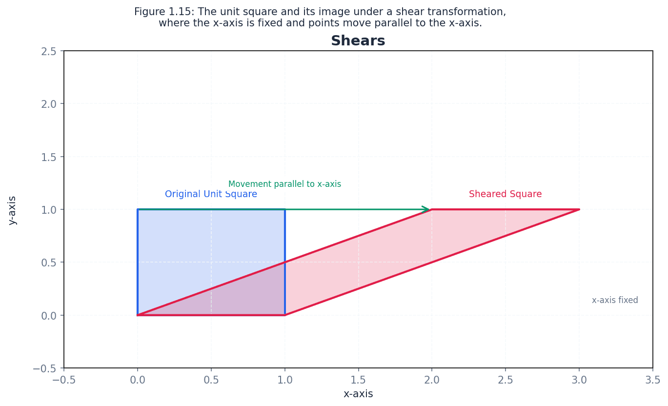
Shear (x-axis fixed)
This matrix represents a shear with the x-axis fixed. Points move parallel to the x-axis.
Shear (y-axis fixed)
This matrix represents a shear with the y-axis fixed. Points move parallel to the y-axis.
shear — A shear is a transformation where points on a fixed line stay the same, and other points move parallel to the fixed line by a distance proportional to their perpendicular distance from the fixed line.
For example, a shear with the x-axis fixed transforms the unit vector j=(0,1) to (k,1), where k is the shear factor. It distorts shapes, turning rectangles into parallelograms. Imagine pushing the top of a stack of cards while keeping the bottom card fixed; the cards slide past each other, creating a slanted stack. This is similar to a shear.
When describing a shear, always state the fixed line (e.g., x-axis fixed) and the image of a point not on the fixed line (e.g., (0,1) mapped to (k,1)).
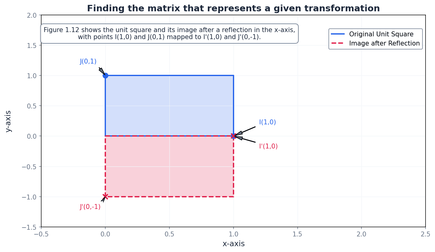
Reflection in x-axis
This matrix reflects a point across the x-axis.
Reflection in y-axis
This matrix reflects a point across the y-axis.
Reflection in line y=x
This matrix reflects a point across the line y=x.
Reflection in line y=-x
This matrix reflects a point across the line y=-x.
Enlargement (centre origin, scale factor k)
This matrix represents an enlargement with the origin as the centre and a scale factor of k.
When multiple transformations are applied one after another, they form a successive transformation. The composite transformation matrix is found by multiplying the individual transformation matrices. Crucially, if transformation B is followed by transformation A, the composite matrix is AB. The order of matrix multiplication is vital here due to its non-commutative nature.
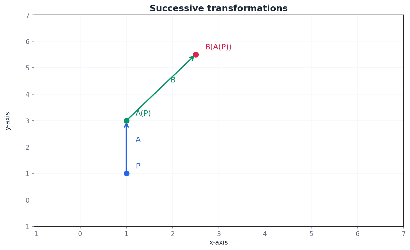
Students often reverse the order of transformations when forming a composite matrix (e.g., for B followed by A, they might write BA instead of AB). Remember that the matrix product AB represents the transformation B followed by A.
For any transformation, certain points or lines may remain unchanged. Points that map to themselves under a transformation are called invariant points. The origin (0,0) is always an invariant point for transformations represented by matrices. An invariant line is a line where the image of every point on that line is also on the same line, though not necessarily the same point.
invariant points — Points that map to themselves under a transformation are called invariant points.
For a point (x, y) to be invariant under a transformation represented by matrix M, M(x, y) must equal (x, y). The origin (0,0) is always an invariant point for transformations represented by matrices. An invariant point is like a pivot in a rotation; it's the only point that doesn't move.
To find invariant points, set M(x, y) = (x, y) and solve the resulting simultaneous equations. If the equations are equivalent, there is a line of invariant points.
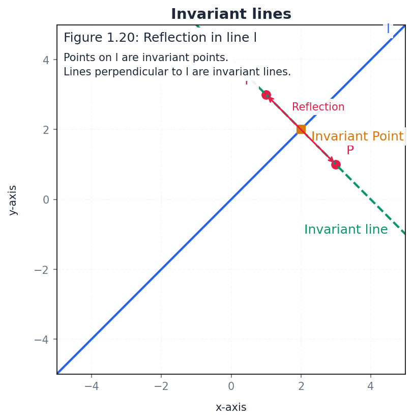
invariant line — A line AB is known as an invariant line under a transformation if the image of every point on AB is also on AB.
It is not necessary for each point on the line to map to itself; it can map to another point on the same line. For example, in a reflection, the mirror line is an invariant line of invariant points, while lines perpendicular to the mirror line are invariant lines but not lines of invariant points. An invariant line is like a track on which a train moves; the train (point) moves, but it stays on the track (line).
Students often confuse invariant lines with lines of invariant points, but actually an invariant line only requires points to map to other points on the same line, not necessarily to themselves.
To find invariant lines, assume the line has the form y = mx + c (or x=k) and apply the transformation, then equate the image line to the original line to solve for m and c.
Use your calculator for matrix operations (addition, subtraction, multiplication) to save time and reduce errors in exams.
Method Frameworks
Common Errors
| Common mistake | How to fix it |
|---|---|
| Assuming matrix multiplication is commutative (AB = BA). | Always remember that matrix multiplication is generally not commutative. The order matters significantly, especially for successive transformations. |
| Attempting to multiply non-conformable matrices. | Before multiplying, always check that the number of columns in the first matrix equals the number of rows in the second matrix. If not, the multiplication is undefined. |
| Reversing the order of matrices for successive transformations. | For transformation B followed by A, the composite matrix is AB. The transformation applied first is on the right. |
| Applying scalar multiplication to only some elements of a matrix. | Ensure every single element within the matrix is multiplied by the scalar number. |
| Confusing invariant lines with lines of invariant points. | An invariant line means points on the line map to other points on the *same* line. A line of invariant points means every point on that line maps *to itself*. |
| Incorrectly stating the order of a matrix. | Always state the order as 'rows × columns', never the other way around. |
Technique Selection
| When you see... | Use... |
|---|---|
| When asked to find the matrix representing a specific geometric transformation (e.g., reflection, rotation, shear). | Find the images of the unit vectors i=(1,0) and j=(0,1) under the transformation. These images will form the columns of the transformation matrix. |
| When describing a transformation given its matrix. | Apply the matrix to the unit vectors i=(1,0) and j=(0,1) to see where they map. This will reveal the nature of the transformation. |
| When dealing with a sequence of transformations (e.g., T1 followed by T2). | Multiply the matrices in reverse order of application: M_composite = M_T2 * M_T1. The matrix for the transformation applied first is on the right. |
| When finding points that do not move under a transformation. | Set the transformation equation M * (x, y) = (x, y) and solve the resulting simultaneous equations for x and y. |
| When finding lines that map onto themselves under a transformation. | Assume the line is y = mx + c (or x=k). Apply the transformation to a general point (x, y) on this line to get (x', y'). Substitute (x', y') into the line equation and compare coefficients to find m and c. |
| When performing any matrix arithmetic (addition, subtraction, multiplication) in an exam. | Use your calculator's matrix functions to perform operations quickly and accurately, especially for larger matrices or to check manual calculations. |
Mark Scheme Notes