Fig 1.6 shows a position-time graph of Amy's journey, with home as the origin. (a) Determine Amy's position at t = 10 min and at t = 30 min from the graph. (b) Calculate Amy's average velocity for the entire journey shown on the graph. (c) Calculate Amy's average speed for the entire journey shown on the graph.
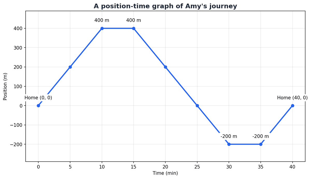
Fig 1.6 shows a position-time graph of Amy's journey, with home as the origin. Fig 1.7 shows a velocity-time graph of Amy's journey. (a) Compare the information presented in Figure 1.6 (position-time) and Figure 1.7 (velocity-time) for Amy's journey between t = 0 min and t = 20 min. (b) Explain how the gradient of Figure 1.6 relates to the values in Figure 1.7. (c) Sketch a possible acceleration-time graph for Amy's journey based on Figure 1.7.
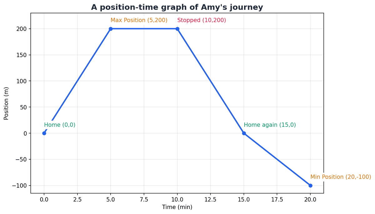
Fig 1.6 shows a position-time graph of Amy's journey, with home as the origin. (a) Calculate Amy's velocity during the first 10 minutes from the graph. (b) Determine the time interval during which Amy is stationary. (c) Calculate Amy's velocity between t = 20 min and t = 30 min. (d) Sketch the corresponding velocity-time graph for Amy's journey based on Figure 1.6.
Fig 1.6 shows a velocity-time graph for an object moving in a straight line. The velocity values at various times are given in the table below:
| Time (s) | Velocity (m s⁻¹) |
|---|---|
| 0 | 0 |
| 2 | 3 |
| 4 | 7 |
| 6 | 9 |
| 8 | 10 |
(a) Calculate an estimate for the distance travelled using the trapezium rule with 4 equal intervals. [4] (b) Assume an estimate using 2 equal intervals for the same data yielded a result of 60 m. Compare the accuracy of using 2 intervals versus 4 intervals for this estimation, and discuss why the difference might be significant. [5]
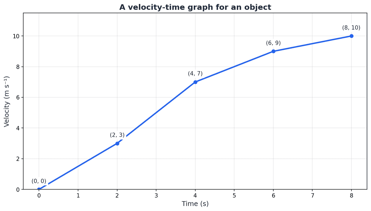
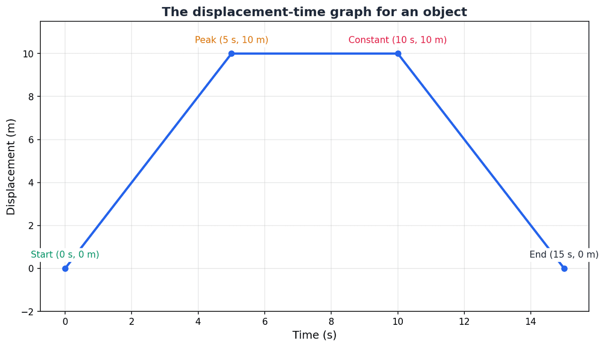
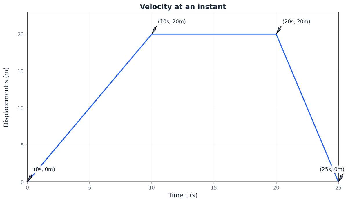
Fig. 1.2 shows the displacement-time graph for an object moving in a straight line. (a) Analyse the features of the displacement-time graph in Fig. 1.2 that indicate a change in velocity. [4] (b) Sketch the corresponding velocity-time graph for the motion shown in Fig. 1.2. [3] (c) Calculate the average velocity of the object over the entire 15 s journey from the displacement-time graph. [3]
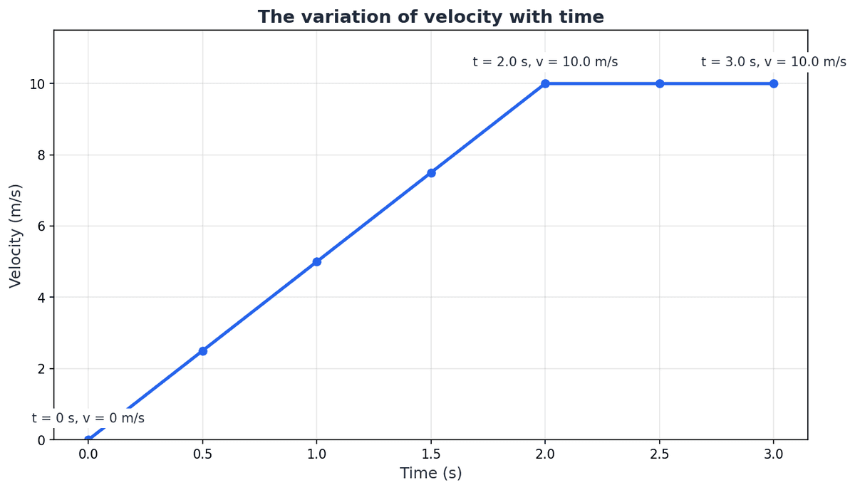
The graph in Fig 1.10 shows the variation of velocity with time for a marble. (a) Calculate the average velocity of the marble between t = 0 s and t = 1.0 s from Figure 1.10. [3] (b) Calculate the average speed of the marble between t = 0 s and t = 1.0 s from Figure 1.10. [3] (c) Compare the average velocity and average speed over the first second, explaining why they are different or similar. [2]
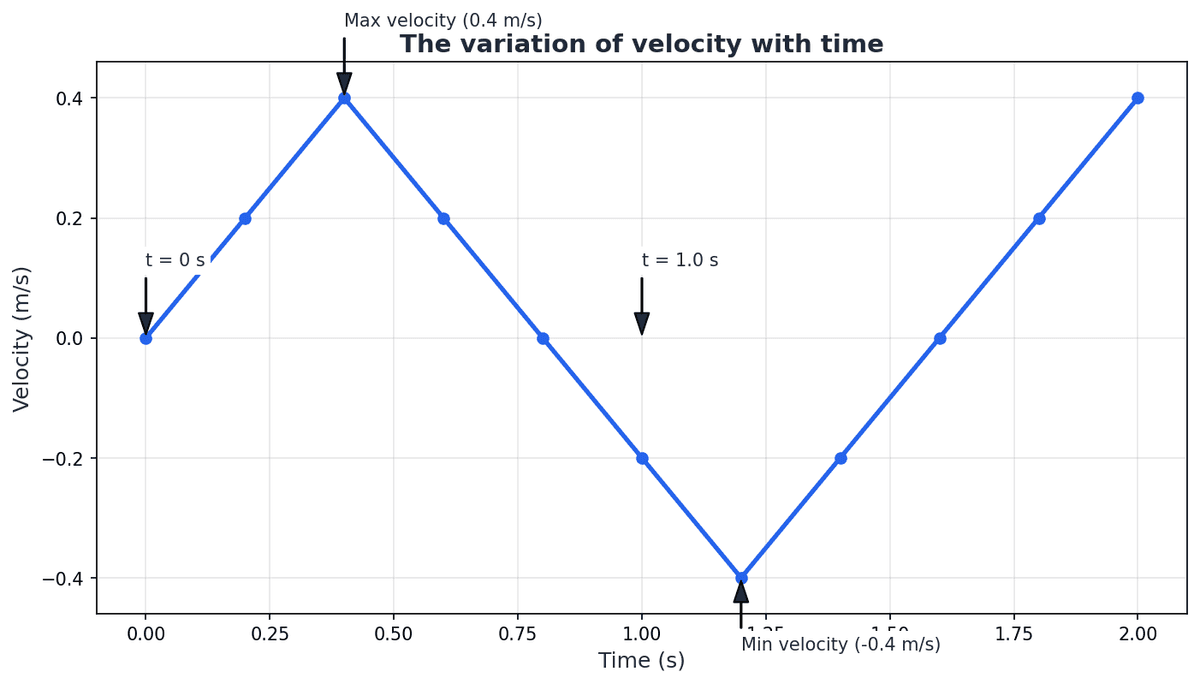
The graph in Fig 1.10 shows the variation of velocity with time for a marble moving in a straight line. (a) Determine the instantaneous velocity of the marble at t = 0.5 s from the graph. [2] (b) Explain what the negative velocity indicates at t = 1.5 s. [3] (c) Calculate the average acceleration of the marble between t = 0.5 s and t = 1.5 s. [3]
Fig 1.2 shows a velocity-time graph for an object moving in a straight line. (a) Discuss the advantages and disadvantages of using graphical estimation methods compared to analytical integration, assuming the velocity function is known. [4] (b) Calculate an estimate for the total distance travelled by the object from t=0s to t=8s, using the trapezium rule with intervals of 2 seconds. [5] (c) Justify whether this estimate is likely to be an overestimate or an underestimate of the actual distance travelled. [3]
The motion of an object is represented by the velocity-time graph shown in Fig 1.1. (a) Calculate the displacement of the object from its initial position at t = 5 s. [4] (b) Compare the total distance travelled by the object with its displacement at t = 5 s. [3]
Fig 1.4 shows a speed-time graph for a runner during a 10-second sprint. (a) Estimate the total distance travelled by the runner from t=0s to t=10s using the trapezium rule with 5 equal intervals. [5] (b) Comment on the accuracy of this estimation given the shape of the graph. [2]
Fig 1.9 shows a position-time graph for a marble moving in a straight line. (a) Estimate the instantaneous velocity of the marble at time t = 1.0 s by drawing a tangent to the curve at point P. [4] (b) Explain how the slope of the position-time graph relates to the marble's velocity. [3] (c) Compare the marble's velocity at t = 0.5 s and t = 1.5 s, stating whether it is increasing or decreasing. [3]
Fig 1.16 shows Hinesh's speed-time graph. (a) Calculate the average acceleration of Hinesh during the first 5 minutes of his journey. (b) Describe Hinesh's motion between t = 5 min and t = 20 min.
Fig 1.16 shows Hinesh's speed-time graph for a 30-minute journey. (a) Calculate the distance Hinesh travels in the first 10 minutes. [3] (b) Calculate Hinesh's average speed for the entire 30-minute journey. [3] (c) State the total time Hinesh spent travelling at a constant speed. [3]
A ball is thrown vertically upwards from the ground. It leaves the hand with an initial velocity of 15 m s⁻¹ and experiences a constant downward acceleration due to gravity of 10 m s⁻². Assume upwards is the positive direction. (a) Draw a velocity-time graph for the ball's motion from the moment it leaves the hand until it hits the ground. Mark the key values on your axes. [3] (b) Calculate the displacement of the ball from its starting point after 5 seconds. [5]
Fig 1.1 shows a velocity-time graph for a rocket during its initial ascent. (a) Estimate the displacement of the rocket during the first 6 seconds using the mid-ordinate rule with 3 equal strips. [4] (b) Analyse how the choice of estimation method (e.g., trapezium rule vs. mid-ordinate rule) might affect the accuracy for this specific curve. [3] (c) Evaluate the limitations of using graphical methods to determine exact displacement. [3]
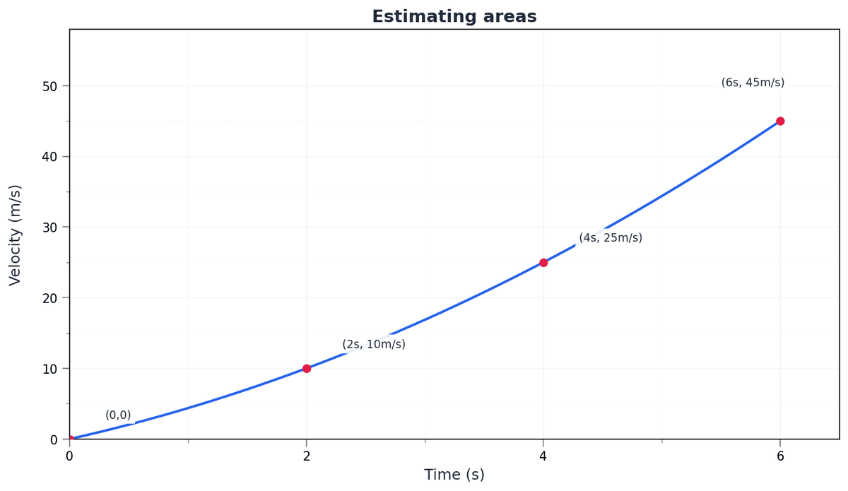
Fig 1.2 shows a displacement-time graph for an object moving in a straight line. (a) Calculate the instantaneous velocity of the object at t = 5 s. [3] (b) Calculate the instantaneous velocity of the object at t = 15 s. [3] (c) Identify the time interval(s) during which the object is at rest. [2]
An object moves in a straight line, and its motion is represented by the velocity-time graph shown in Fig. 1.1. (a) Determine the velocity of the object at t = 2 s and at t = 8 s from Fig. 1.1. [4] (b) State what a horizontal line on a velocity-time graph represents. [3]
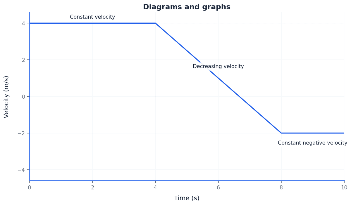
Fig 1.20 shows Sunil's velocity-time graph for a 10-second journey. (a) Calculate Sunil's displacement from t = 0 s to t = 6 s. [3] (b) Calculate Sunil's final displacement at t = 10 s. [4] (c) Compare the total distance travelled with the final displacement for Sunil's journey, explaining any difference. [3]
Fig 1.1 illustrates the position of a marble relative to a hand. The hand is at the zero position, and the positive direction is upwards. (a) State the initial positive position of the marble shown in Fig 1.1. [1] (b) The marble then moves to a new position of -0.5 m. Calculate the displacement of the marble. [2] (c) Explain the meaning of a negative position value in the context of this diagram. [2]
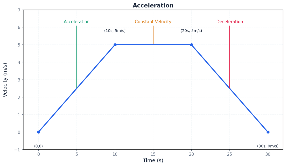
Fig 1.2 shows a velocity-time graph for a cyclist. (a) Calculate the acceleration of the cyclist during the first 10 seconds. [3] (b) Calculate the acceleration of the cyclist between t = 20 s and t = 30 s. [3] (c) Describe the motion of the cyclist between t = 10 s and t = 20 s. [3]
When analysing motion, it is sometimes necessary to determine displacement from a velocity-time graph where the velocity changes non-linearly. (a) Describe one method for estimating the area under a non-linear velocity-time graph. [3] (b) State why estimation methods are sometimes necessary for such graphs. [2]
An object's motion can be described in terms of its displacement, velocity, and acceleration. These are all vector quantities. (a) Discuss the importance of specifying a positive direction when working with vector quantities in mechanics. [6] (b) Determine the resultant displacement of an object that moves 5 km East, then 3 km West, assuming East is the positive direction. [4]
When describing motion, it is important to distinguish between different types of physical quantities. (a) Explain the difference between scalar and vector quantities, using examples relevant to motion. [4] (b) Identify which of the following are vector quantities: speed, distance, velocity, acceleration. [3]
A train travels in a straight line. It moves for 40 seconds at a constant velocity of 20 m s⁻¹ in the positive direction. It then reverses direction and travels for 60 seconds at a constant velocity of 10 m s⁻¹. The total duration of the motion is 100 seconds. (a) Calculate the total distance travelled by the train during the 100 seconds. [5] (b) Explain why the magnitude of the displacement is less than the total distance travelled in this scenario. [4]
Fig. 1.1 shows the velocity-time graph for an object moving in a straight line. (a) Describe the motion of the object shown in Fig. 1.1 from t=0 s to t=10 s. [3] (b) Calculate the displacement of the object from t=0 s to t=10 s. [5]
An object moves in a straight line. (a) Define the term 'displacement'. [2] (b) Calculate the distance travelled by an object with a constant speed of 15 m s⁻¹ for 5 seconds. [2]
Fig 1.12 shows the velocity-time graph for a marble moving in a straight line. (a) Calculate the acceleration of the marble between t = 0 s and t = 1 s. (b) Calculate the acceleration of the marble between t = 1 s and t = 2 s. (c) Explain what the negative acceleration means in this context.
A runner completes a 400 m race. They accelerate uniformly from rest for 5 seconds, reaching a maximum speed of 8 m/s. They maintain this speed for a further 30 seconds before decelerating uniformly to a stop in 5 seconds. (a) Draw a velocity-time graph for the runner's motion, labelling all significant points. [5] (b) Calculate the total displacement of the runner. [4] (c) Explain how the graph would change if the runner had decelerated over a shorter time period at the end of the second phase. [2]
A car's motion is represented by the speed-time graph shown in Fig. 1.4. (a) Interpret the motion of the object between t=5 s and t=10 s from Fig. 1.4. [3] (b) Calculate the total distance travelled by the object from t=0 s to t=10 s. [4]
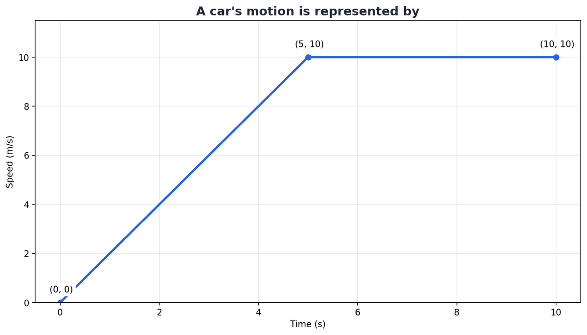
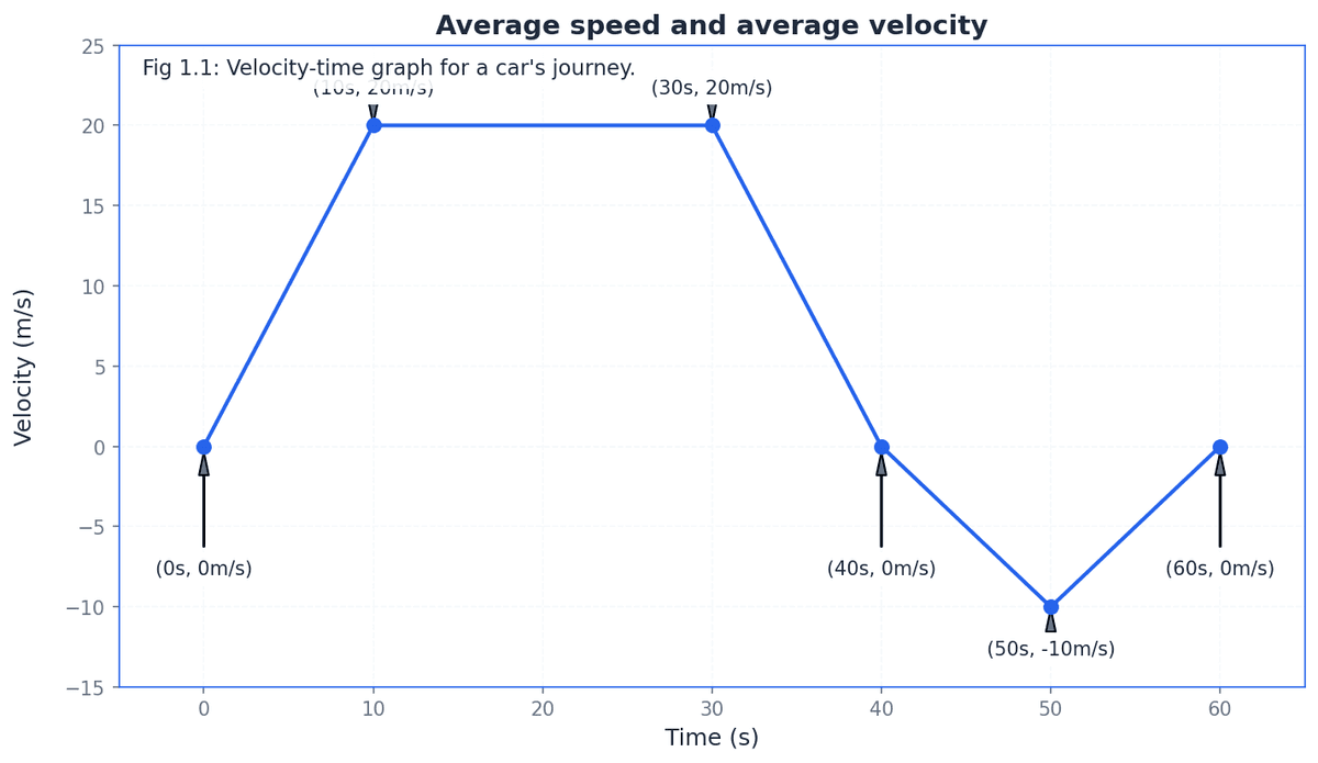
Fig 1.1 shows a velocity-time graph for a car's journey. (a) Calculate the total distance travelled by the car. [4] (b) Calculate the average speed of the car for the entire journey. [2] (c) Interpret the significance of the negative velocity shown in the graph. [3]
A car accelerates from an initial velocity of 15 m s⁻¹ to a final velocity of 5 m s⁻¹ in a straight line over a period of 4 seconds. (a) Calculate the acceleration of the car. [3] (b) Explain what a negative acceleration implies about the car's motion. [4]
Understanding how to interpret graphs is crucial in mechanics. (a) State what the area under a velocity-time graph represents. [2] (b) Calculate the displacement of an object that moves at a constant velocity of 5 m s⁻¹ for 10 seconds. [3]
The graph in Fig 1.10 shows the variation of velocity with time for a marble. (a) Calculate the acceleration of the marble at t = 1.0 s from Figure 1.10. (b) Interpret the meaning of the constant gradient in Figure 1.10.
A ball is dropped from rest from a height of 20 m. Assume air resistance is negligible and the acceleration due to gravity is 9.81 m s⁻². (a) Calculate the instantaneous velocity of the ball just before it hits the ground. [3] (b) Compare this instantaneous velocity with its average velocity during the fall. [3]
Motion in a straight line can be represented graphically. (a) State two types of graphs commonly used to represent motion in a straight line. [2] (b) Sketch a displacement-time graph for an object moving with constant positive velocity. [3]
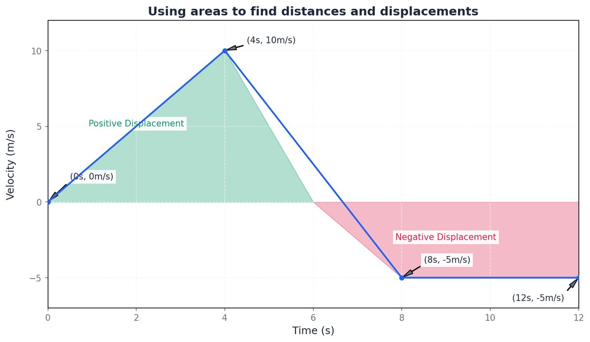
Fig 1.3 shows a velocity-time graph for an object's motion. (a) Derive the formula for the area of a trapezium, given its parallel sides are velocities V₁ and V₂ and the time interval is T, relating it to displacement. [4] (b) Explain why, for a velocity-time graph, the total distance travelled may differ from the final displacement. [3] (c) Calculate the average speed of the object over the entire 12-second journey shown in Fig 1.3. [4]
A rocket launches vertically upwards from rest. It accelerates uniformly to a velocity of 150 m s⁻¹ in the first 5 seconds. After this, its engines cut out, and it continues to move upwards under gravity, reaching its maximum height at 15 seconds from launch. Assume g = 9.81 m s⁻². (a) Calculate the acceleration of the rocket in the first 5 seconds. [3] (b) Determine the average acceleration of the rocket during the entire 15 seconds. [5]
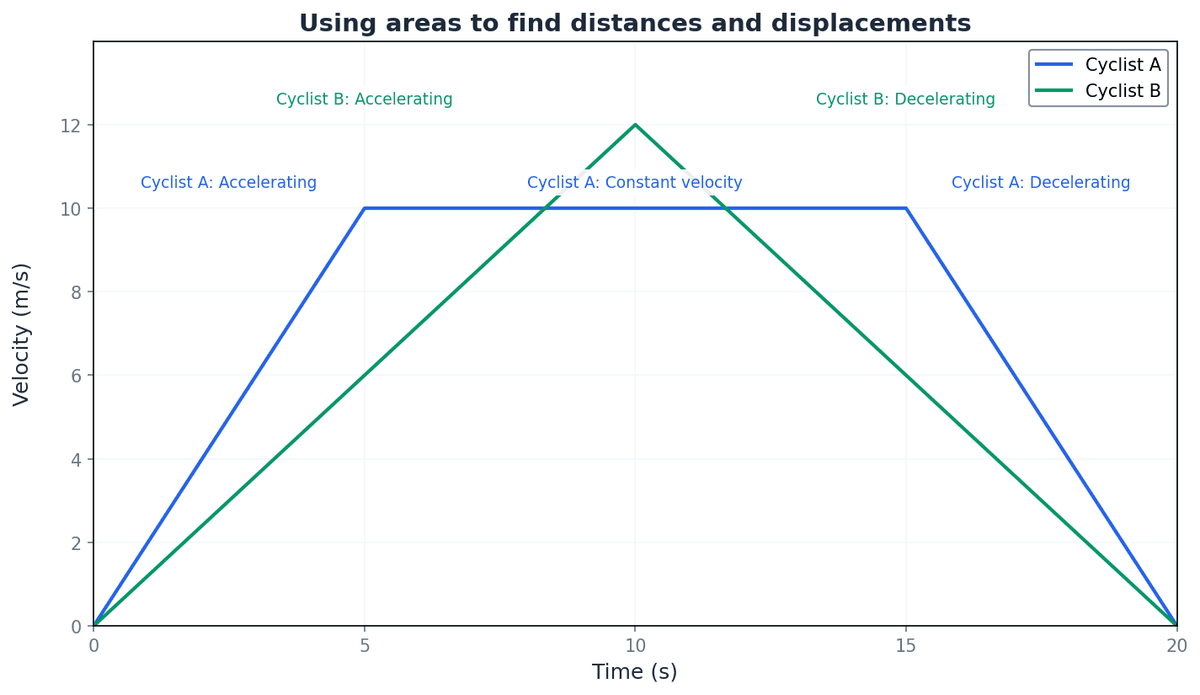
Fig 1.4 shows two velocity-time graphs on the same axes for Cyclist A and Cyclist B, both starting from rest. (a) Analyse the motion of the two cyclists, A and B, by describing their acceleration and deceleration phases. [5] (b) Compare the total displacement of Cyclist A and Cyclist B after 20 seconds. [4] (c) Evaluate which cyclist had the greater average speed over the first 15 seconds. [3]
A car accelerates from rest, reaching a velocity of 10 m s⁻¹ after 4 seconds. It then continues to accelerate, reaching 15 m s⁻¹ after a further 4 seconds (total time 8 seconds). The acceleration is not constant during either interval. (a) Sketch a velocity-time graph for the car's motion. [3] (b) Estimate the total distance travelled by the car using the trapezium rule with two equal time intervals. [3] (c) Suggest how the accuracy of the estimation could be improved. [2]
Fig 1.19 shows Sunil's speed-time graph for a 10-second journey. (a) Calculate Sunil's total distance travelled during the 10 seconds. [3] (b) Calculate Sunil's average speed for the entire journey. [3] (c) Determine the maximum speed Sunil reaches during his journey. [2]