Nexelia Academy · Official Revision Notes
Complete A-Level revision notes · 6 chapters
This chapter introduces hypothesis testing as a statistical method to analyze data and reach conclusions about claims. It covers understanding key terms like null and alternative hypotheses, significance level, critical region, and test statistic. Students learn to formulate hypotheses and perform tests using direct binomial probabilities or normal approximations, interpreting results in context.
null hypothesis — In a hypothesis test, the claim is called the null hypothesis, abbreviated to H0.
The null hypothesis is the initial assumption that there is no difference or no effect, representing the status quo or a commonly accepted belief. It is expressed in terms of a population parameter, such as a probability or a mean value, and is the hypothesis that is tested directly. In a courtroom, the null hypothesis is that the defendant is innocent. The prosecution tries to find enough evidence to reject this hypothesis.
Students often think the null hypothesis is what the researcher wants to prove, but actually it's the statement of no effect or no difference that the researcher tries to disprove.
Always state the null hypothesis (H0) using an equality sign (e.g., p = 0.4 or μ = 10) and ensure it refers to a population parameter, not a sample statistic.
alternative hypothesis — If you are not going to accept the null hypothesis, then you must have an alternative hypothesis to accept; the alternative hypothesis abbreviation is H1.
The alternative hypothesis is the statement that contradicts the null hypothesis, suggesting that there is a difference, an effect, or a specific direction of change. It is accepted if there is sufficient evidence to reject the null hypothesis. If the null hypothesis is that a coin is fair, the alternative hypothesis could be that the coin is biased (two-tailed) or specifically biased towards heads (one-tailed).
Students often think H1 must always be 'not equal to', but actually it can be 'less than' or 'greater than' depending on the direction of the claim being tested (one-tailed vs. two-tailed).
Ensure the alternative hypothesis (H1) is consistent with the claim being investigated (e.g., p < 0.4, p > 0.4, or p ≠ 0.4) and refers to the same population parameter as H0.
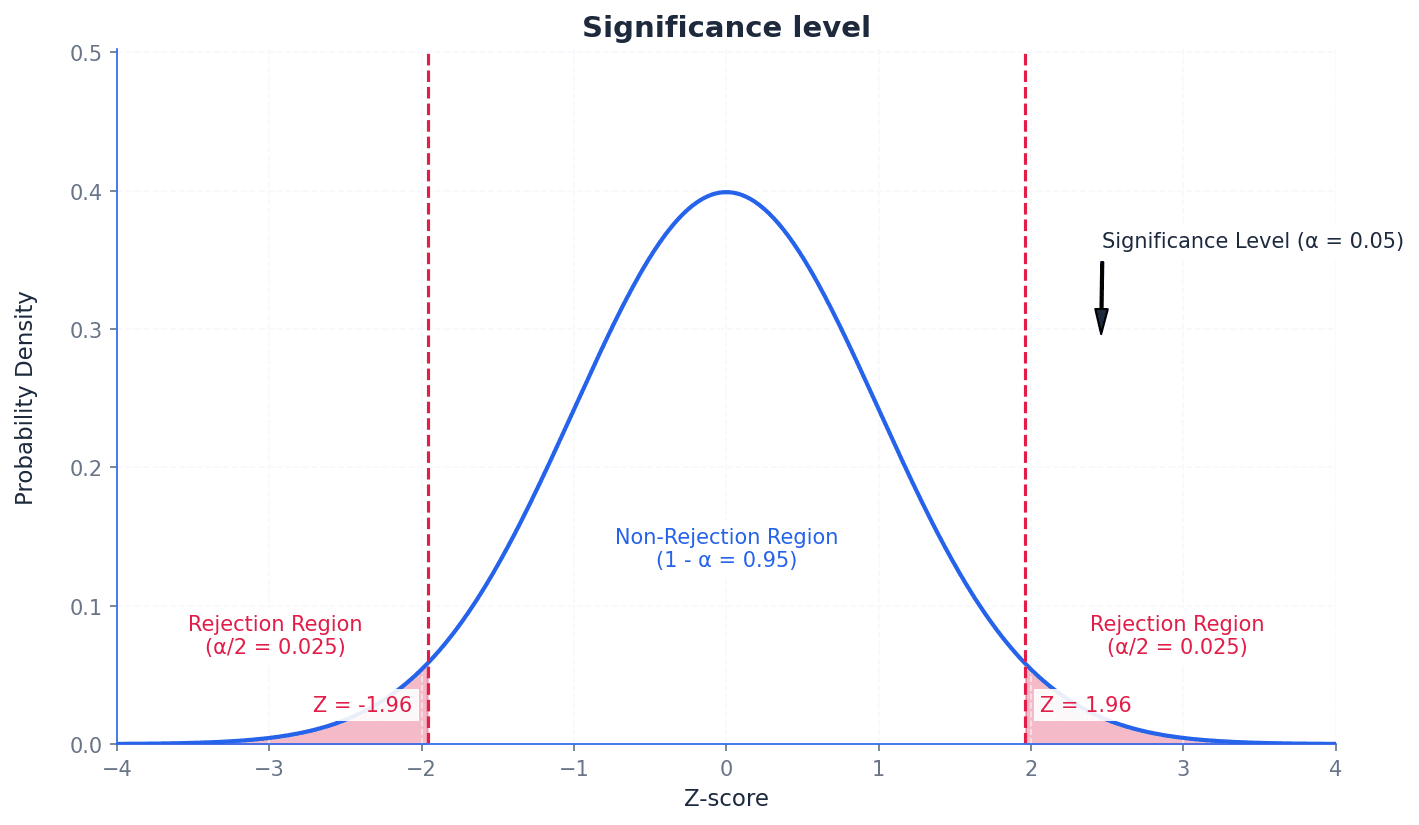
significance level — The percentage value of 5% is known as the significance level.
The significance level, often denoted by α, is the probability of rejecting the null hypothesis when it is actually true (a Type I error). It determines the threshold for statistical significance, defining how small a probability must be for a result to be considered unlikely to occur by chance. Imagine a quality control check where you set a 'tolerance level' for defects. If the defect rate exceeds this level, you reject the batch. The significance level is like this tolerance level for rejecting a claim.
Students often think a 5% significance level means there's a 5% chance the alternative hypothesis is true, but actually it means there's a 5% chance of incorrectly rejecting a true null hypothesis.
Always state the chosen significance level (e.g., 5% or 0.05) at the beginning of your hypothesis test and use it consistently to compare with your calculated p-value or critical region.
test statistic — The test statistic is the calculated probability using sample data in a hypothesis test.
The test statistic is a value calculated from the sample data during a hypothesis test. This value is then compared to the critical region or used to find a p-value, which helps in deciding whether to reject or accept the null hypothesis. If you're testing a new recipe, the 'test statistic' is the taste score given by a sample of tasters. You compare this score to a benchmark to decide if the recipe is better.
Students often confuse the test statistic with the critical value, but actually the test statistic is calculated from the sample data, while the critical value is determined by the significance level and distribution.
critical region — The range of values at which you reject the claim is the critical region or rejection region.
The critical region is the set of values of the test statistic for which the null hypothesis is rejected. Its size is determined by the significance level, and it can be located in one tail (one-tailed test) or both tails (two-tailed test) of the distribution. Think of a target board. The bullseye is the 'acceptance region', but if your arrow lands outside a certain ring (the critical region), you 'reject' the idea that you hit the target accurately.
rejection region — The range of values at which you reject the claim is the critical region or rejection region.
The rejection region is another name for the critical region, representing the set of outcomes for which the null hypothesis is rejected. If the calculated test statistic falls within this region, the null hypothesis is rejected in favor of the alternative hypothesis. In a game, if your score falls into a certain 'danger zone' (rejection region), you lose. Otherwise, you continue playing (accept the null hypothesis).
Students often think the critical region is where the alternative hypothesis is true, but actually it's the region where the observed data is so extreme that it provides strong evidence against the null hypothesis.
Clearly define the critical region in terms of the test statistic (e.g., X ≤ 1 or X ≥ 12) and ensure it corresponds to the direction of the alternative hypothesis and the chosen significance level.
critical value — The value at which you change from accepting to rejecting the claim is the critical value.
The critical value is the boundary point(s) of the critical region. If the test statistic falls beyond this value (into the critical region), the null hypothesis is rejected. It is determined by the significance level and the distribution of the test statistic. Imagine a 'pass/fail' mark on an exam. If your score (test statistic) is below that mark (critical value), you fail (reject the null hypothesis).
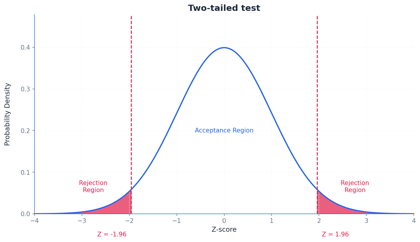
acceptance region — The other region of the graph is the acceptance region.
The acceptance region is the set of values of the test statistic for which the null hypothesis is not rejected. If the calculated test statistic falls within this region, there is insufficient evidence to reject the null hypothesis. If a product passes a quality check (its measurements fall within acceptable limits), it's in the 'acceptance region'. If it's outside, it's rejected.
Students often think 'accepting' the null hypothesis means it's proven true, but actually it just means there isn't enough evidence to reject it; it doesn't confirm its truth.
Hypothesis testing is a statistical method used to analyze data and draw conclusions about claims regarding a population parameter. It involves setting up two opposing statements: the null hypothesis (H0), which represents the status quo or no effect, and the alternative hypothesis (H1), which contradicts H0. The goal is to determine if there is sufficient evidence from sample data to reject H0 in favour of H1.
The nature of the alternative hypothesis determines whether a test is one-tailed or two-tailed. A one-tailed test is used when H1 specifies a direction (e.g., a probability is less than or greater than a certain value). A two-tailed test is used when H1 suggests a difference in either direction (e.g., a probability is not equal to a certain value). For two-tailed tests, the significance level is split equally between the two tails of the distribution.
Incorrectly choosing between a one-tailed and two-tailed test; the choice depends on whether the claim specifies a direction (increase/decrease) or just a difference.
When dealing with a single observation from a binomial distribution, hypothesis tests can be carried out using direct probability evaluation. This involves calculating the probability of observing the sample data (or more extreme data) under the assumption that the null hypothesis is true. This calculated probability, often referred to as the p-value, is then compared to the significance level to make a decision about H0.
For large sample sizes, a binomial distribution can be approximated by a normal distribution. This approximation simplifies calculations, especially when direct binomial probability evaluation becomes cumbersome. When using a normal approximation, it is crucial to apply a continuity correction to account for the discrete nature of the binomial distribution being approximated by a continuous normal distribution.
Forgetting to apply continuity correction when approximating a binomial distribution with a normal distribution.
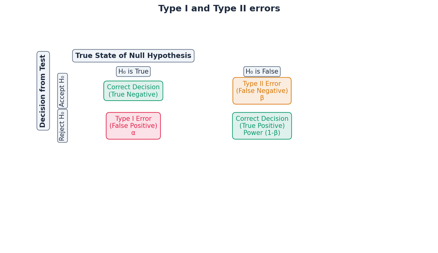
Type I error — A Type I error occurs when a true null hypothesis is rejected.
A Type I error happens when the null hypothesis is true, but based on the sample data, we incorrectly reject it. The probability of making a Type I error is equal to the significance level (α) of the test. In a courtroom, a Type I error is when an innocent person is found guilty.
Type II error — A Type II error occurs when a false null hypothesis is accepted.
A Type II error happens when the null hypothesis is false, but based on the sample data, we incorrectly fail to reject it. The probability of making a Type II error is denoted by β and is harder to calculate as it depends on the true value of the population parameter under the alternative hypothesis. In a courtroom, a Type II error is when a guilty person is found innocent.
Confusing Type I and Type II errors, or their probabilities (significance level vs. beta).
When asked to explain a Type I error in context, state that it is concluding the alternative hypothesis is true when the null hypothesis is actually true, without using H0 or H1 in the explanation.
To calculate the probability of a Type II error, you need to assume a specific true value for the population parameter under the alternative hypothesis, which is often provided in the question.
Always state your null (H0) and alternative (H1) hypotheses clearly in terms of the population parameter (e.g., p).
Ensure your conclusion is stated in context, avoiding definitive language like 'proven' and instead using phrases like 'there is sufficient evidence to suggest...'.
When using a normal approximation, explicitly state the distribution used (e.g., X ~ N(np, npq)) and show the continuity correction.
Exam Technique
Hypothesis test for binomial distribution (direct probability)
Hypothesis test for binomial distribution (normal approximation)
| Mistake | Fix |
|---|---|
| Confusing the null hypothesis with what the researcher wants to prove. | Remember H0 is the statement of no effect or no difference, which the researcher tries to disprove. |
| Incorrectly choosing between a one-tailed and two-tailed test. | The choice depends on whether the claim specifies a direction (e.g., 'less than', 'greater than') or just a general difference ('not equal to'). |
| Forgetting to apply continuity correction when using a normal approximation. | Always adjust the discrete value by ±0.5 when converting from a discrete (binomial) to a continuous (normal) distribution. |
This chapter introduces the Poisson distribution as a discrete probability model for events occurring randomly and independently within a fixed interval. It covers calculating probabilities, adapting the distribution for different intervals, and using it to approximate binomial and normal distributions. Finally, it details hypothesis testing for Poisson models, including understanding Type I and Type II errors.
Poisson distribution — A discrete probability distribution used to model situations where events occur singly, at random, and independently in a given interval of space or time.
This distribution is characterized by a single parameter, \(\lambda\) (lambda), which represents both its mean and variance. It is suitable for rare events over a fixed interval, unlike binomial or geometric distributions which count successes in trials. Imagine counting the number of meteor showers visible from your town in a year; they happen randomly, one at a time, and independently. The Poisson distribution helps predict the probability of seeing a certain number of showers.
Students often think the Poisson distribution is only for events over time, but it actually can also model events occurring in a fixed interval of space, such as defects per metre of pipe or bubbles in glassware.
Parameter — A numerical characteristic of a population or a probability distribution.
For a Poisson distribution, the single parameter is \(\lambda\) (lambda), which defines the mean and variance of the distribution. This parameter is crucial for calculating probabilities and understanding the distribution's shape. Think of a recipe for a cake; the amount of sugar (a parameter) determines how sweet the cake will be. Similarly, \(\lambda\) determines the 'sweetness' (mean and spread) of the Poisson distribution.
Students often think that the mean and variance are always different values, but for a Poisson distribution, the mean and variance are equal, both represented by the parameter \(\lambda\).
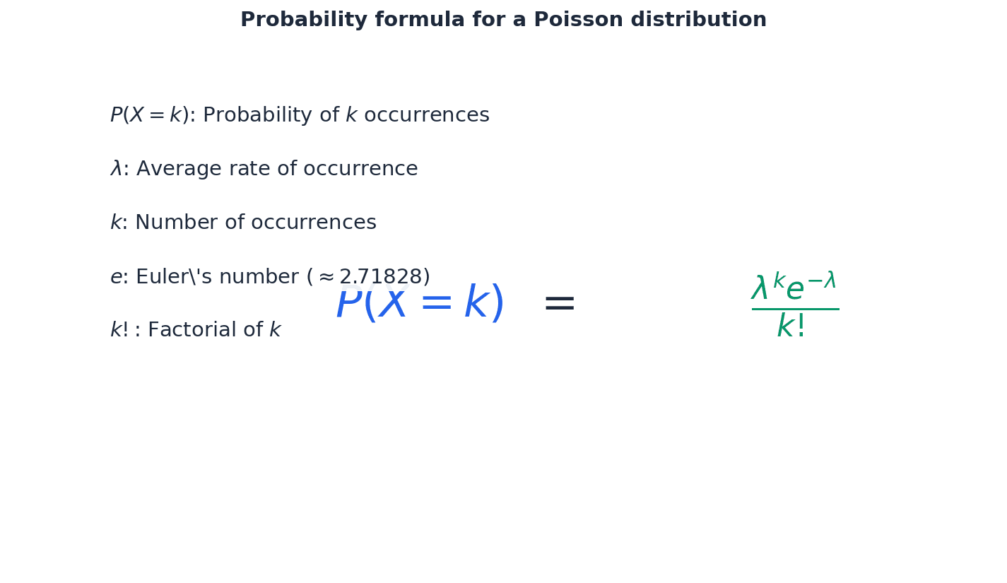
Poisson Probability Formula
Used to calculate the probability of exactly 'r' events occurring in a fixed interval for a Poisson distribution. Valid for r = 0, 1, 2, 3, ...
Poisson Mean
The expected value (mean) of a Poisson distribution is equal to its parameter \(\lambda\).
Poisson Variance
The variance of a Poisson distribution is equal to its parameter \(\lambda\), and thus equal to its mean.
The Poisson distribution models discrete events that occur singly, independently, and at random within a fixed interval of time or space. A key characteristic is that its mean and variance are both equal to its single parameter, \(\lambda\). When asked to state assumptions for a Poisson model, it is crucial to explicitly mention that 'events occur singly, at random, and independently' and 'at a constant average rate' to secure full marks.
When asked to state assumptions for a Poisson model, explicitly mention 'events occur singly, at random, and independently' and 'at a constant average rate' to secure full marks.
The parameter \(\lambda\) represents the mean number of events in a *given* interval. If the interval of time or space changes, the parameter \(\lambda\) must be adjusted proportionally. For example, if the mean rate is 2 events per 5 minutes, then for a 10-minute period, \(\lambda\) would be 4, and for a 1-minute period, \(\lambda\) would be 0.4. This ensures the model accurately reflects the expected number of events in the new interval.
Students often forget to adjust the Poisson parameter \(\lambda\) when the interval of time or space changes.
The Poisson distribution can serve as an approximation to the binomial distribution, \(B(n, p)\), under specific conditions. This approximation is valid when the number of trials, \(n\), is large, and the probability of success, \(p\), is small. In such cases, the Poisson parameter \(\lambda\) is set equal to \(np\), the mean of the binomial distribution. This approximation simplifies calculations for situations with many trials and rare events.
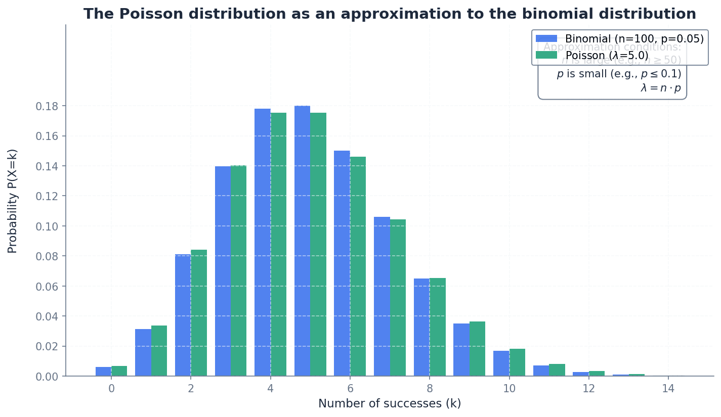
Students often misinterpret the conditions for approximating a binomial distribution with a Poisson distribution; remember that \(n\) must be large, \(p\) small, and \(np\) moderate.
Continuity correction — An adjustment applied when approximating a discrete probability distribution with a continuous one, typically by extending the discrete value by 0.5 in either direction.
Since a Poisson distribution is discrete and a normal distribution is continuous, a continuity correction is necessary to account for the difference in how probabilities are calculated. For example, \(P(X=r)\) in a discrete distribution becomes \(P(r-0.5 < Y < r+0.5)\) in a continuous approximation. Imagine trying to measure the height of discrete steps (Poisson) with a continuous ruler (Normal); you have to measure the range it covers, from halfway below to halfway above, to get an accurate representation.
When the parameter \(\lambda\) of a Poisson distribution is large (typically \(\lambda > 15\)), the Poisson distribution can be approximated by a normal distribution, \(N(\lambda, \lambda)\). This approximation is particularly useful for calculating probabilities involving ranges of values. Due to the discrete nature of the Poisson and the continuous nature of the normal distribution, a continuity correction must always be applied when using this approximation.
Students often forget to apply a continuity correction when using the normal distribution as an approximation to the Poisson distribution.
Always apply a continuity correction when using the normal approximation for a Poisson distribution in hypothesis testing or probability calculations, as failing to do so will lead to inaccurate results and loss of marks.
Hypothesis testing — A statistical method used to determine if there is enough evidence in a sample data to infer that a certain condition is true for the entire population.
It involves formulating a null hypothesis (H0) and an alternative hypothesis (H1), calculating a test statistic, and comparing it to a critical value or p-value to decide whether to reject H0. For Poisson distributions, this often involves testing changes in the mean rate \(\lambda\). Think of a court trial: the null hypothesis is 'innocent until proven guilty'. You collect evidence (data) to see if there's enough to reject 'innocent' and conclude 'guilty' (the alternative hypothesis).
Type I error — An error that occurs when the null hypothesis is incorrectly rejected when it is actually true.
This means concluding that there is a significant effect or change when, in reality, there isn't one. The probability of a Type I error is equal to the significance level (\(\alpha\)) of the test. In a court trial, a Type I error is convicting an innocent person; the system concluded guilt when the person was actually innocent.
When asked to explain a Type I error in context, describe what it means specifically for the scenario given (e.g., concluding the mean rate has fallen when it hasn't) and state its probability as the significance level.
Type II error — An error that occurs when the null hypothesis is incorrectly accepted when it is actually false.
This means failing to detect a significant effect or change that truly exists. The probability of a Type II error is denoted by \(\beta\) and is harder to calculate without knowing the true alternative parameter value. In a court trial, a Type II error is letting a guilty person go free; the system failed to conclude guilt when the person was actually guilty.
Students often think that 'accepting the null hypothesis' means it is proven true, but it actually means there is insufficient evidence to reject it, not that it is definitively true.
When conducting a hypothesis test, clearly state the null and alternative hypotheses (H0 and H1), the significance level, whether it's a one-tailed or two-tailed test, and provide a contextual interpretation of your conclusion.
Clearly state the distribution and its parameter (e.g., X ~ Po(\(\lambda\))) at the start of your solution.
For approximation questions, explicitly state the conditions met for the approximation to be valid.
Exam Technique
Calculating Poisson Probabilities
Poisson Approximation to Binomial
| Mistake | Fix |
|---|---|
| Forgetting to adjust the Poisson parameter \(\lambda\) when the interval of time or space changes. | Always re-read the question carefully to identify the interval for which the probability is required and adjust \(\lambda\) proportionally from the given average rate. |
| Failing to apply a continuity correction when using the normal approximation for a Poisson distribution. | Remember that Poisson is discrete and Normal is continuous. For \(P(X=r)\) use \(P(r-0.5 < Y < r+0.5)\), for \(P(X \le r)\) use \(P(Y < r+0.5)\), and for \(P(X \ge r)\) use \(P(Y > r-0.5)\). |
| Confusing 'accepting the null hypothesis' with proving it true. | Always state that there is 'insufficient evidence to reject the null hypothesis' rather than 'accepting' it, as a lack of evidence does not equate to proof. |
This chapter focuses on determining the mean and variance of linear combinations of random variables. It covers both single random variables and combinations of independent variables, including specific rules for Normal and Poisson distributions, emphasizing that variances are always added for independent variables.
Understanding linear combinations of random variables is crucial for solving problems where quantities are combined or scaled. This chapter details how to find the expectation (mean) and variance of such combinations, which is essential for calculating probabilities and making predictions about combined outcomes. We will explore rules for both single random variables and for sums and differences of independent random variables.
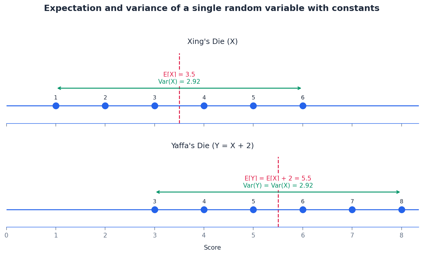
When a random variable X is transformed by a linear combination aX + b, its expectation and variance change in predictable ways. The constant 'a' scales both the expectation and the variance, while the constant 'b' only affects the expectation, shifting it without changing the spread of the distribution. These rules apply universally to any random variable X.
Expectation of a linear combination of a random variable
Applies to any random variable X and constants a, b. The expectation is scaled by 'a' and shifted by 'b'.
Variance of a linear combination of a random variable
Applies to any random variable X and constants a, b. The constant 'b' does not affect the variance, and the constant 'a' is squared when multiplying the variance.
Students often think that Var(aX + b) = a Var(X) + b, but actually Var(aX + b) = a^2 Var(X). Remember that adding a constant does not change the spread of the data, only its location, and scaling affects variance by the square of the scaling factor.
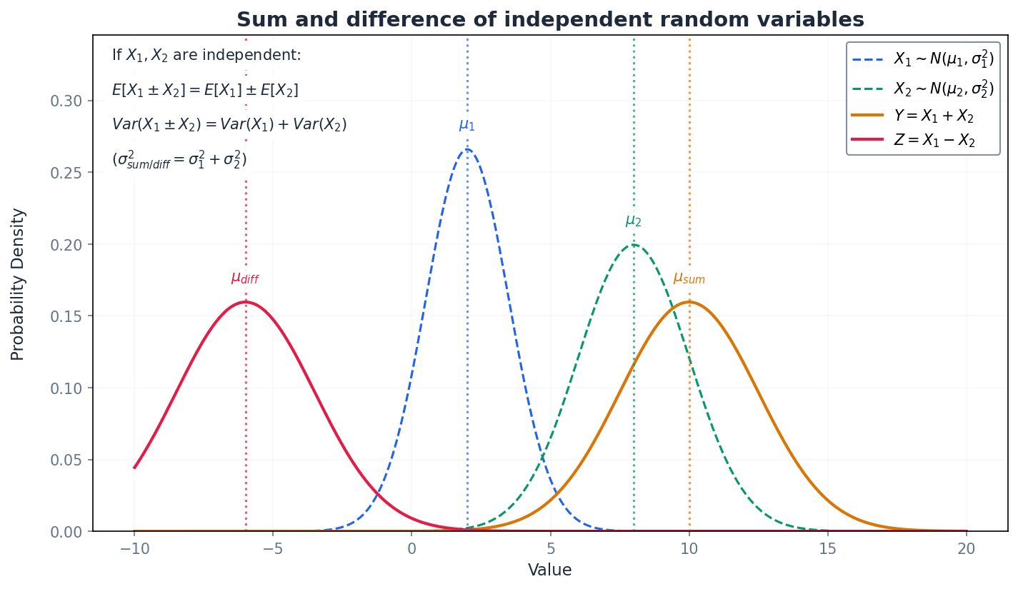
When combining two or more independent random variables, specific rules govern the expectation and variance of their sum or difference. A crucial point is that for independent variables, variances are always added, regardless of whether the variables themselves are being added or subtracted. This reflects that combining independent sources of variability always increases the overall uncertainty.
Expectation of the sum of two independent random variables
Applies to any two independent random variables X and Y. The expectation of the sum is the sum of the individual expectations.
Expectation of the difference of two independent random variables
Applies to any two independent random variables X and Y. The expectation of the difference is the difference of the individual expectations.
Variance of the sum of two independent random variables
Applies to any two independent random variables X and Y. Variances are always added when combining independent random variables.
Variance of the difference of two independent random variables
Applies to any two independent random variables X and Y. Variances are always added when combining independent random variables, even for differences.
Students often think that Var(X - Y) = Var(X) - Var(Y), but actually Var(X - Y) = Var(X) + Var(Y). This is a common trap; remember that variances are always added for independent random variables because combining independent sources of variation always increases overall variability.
Expectation of a linear combination of two independent random variables
Applies to any two independent random variables X and Y and constants a, b. This rule can be extended to any number of independent random variables.
Variance of a linear combination of two independent random variables
Applies to any two independent random variables X and Y and constants a, b. This rule can be extended to any number of independent random variables, and variances are always added.
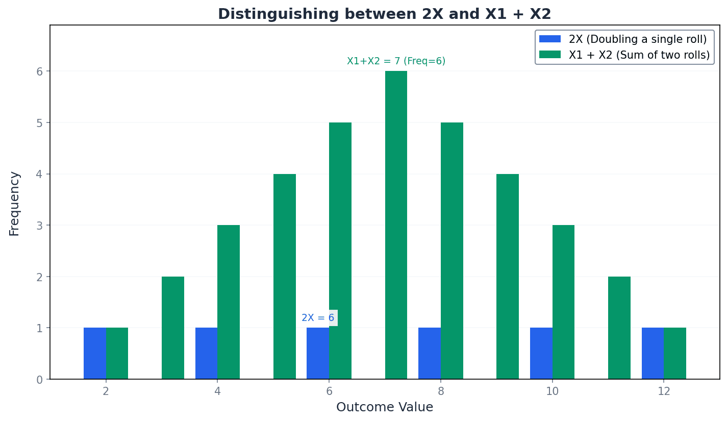
It is crucial to differentiate between scaling a single random variable (aX) and summing multiple independent observations of the same random variable (X1 + X2 + ... + Xn). While their expectations might be the same, their variances differ significantly. For example, E(2X) = E(X1 + X2) = 2E(X), but Var(2X) = 4Var(X) whereas Var(X1 + X2) = 2Var(X).
Students often confuse 2X (twice the size of an observation from X) with X1 + X2 (the sum of two independent observations of X). Remember that E(2X) = E(X1 + X2) but Var(2X) = 4Var(X) while Var(X1 + X2) = 2Var(X).
A key property of Normal distributions is that any linear combination of independent Normal random variables will also result in a Normal distribution. This allows us to calculate probabilities for these new combined variables by finding their new mean and variance, and then standardizing to a Z-score using the standard normal distribution tables. This is particularly useful in practical problems involving combined measurements.
For Poisson distributions, a specific rule applies to their sum. If X and Y are independent Poisson distributions, their sum X+Y also follows a Poisson distribution. However, this property does not extend to all linear combinations. Only the sum of independent Poisson distributions results in a Poisson distribution; other combinations like 2X+Y will not, as their mean and variance will not be equal, which is a requirement for a Poisson distribution.
Sum of independent Poisson distributions
If X and Y have independent Poisson distributions, their sum X+Y also has a Poisson distribution with a mean equal to the sum of their individual means. This can be extended to any number of independent Poisson distributions.
Students often think that any linear combination of Poisson distributions will result in a Poisson distribution, but actually only the sum of independent Poisson distributions (X+Y) results in a Poisson distribution; combinations like 2X+Y do not, as their mean and variance will not be equal.
Clearly state the distribution and its parameters for any new random variable formed by a linear combination, especially for Normal and Poisson distributions. This helps in organizing your solution and ensures you apply the correct subsequent steps.
When solving problems, break down complex linear combinations into smaller steps, calculating expectation and variance separately. This systematic approach reduces errors and makes your working clearer.
Always check for independence between random variables before applying variance rules for sums/differences. The rules for adding variances only hold for independent variables.
Pay close attention to whether a question refers to 'n times a single observation' (nX) or 'the sum of n independent observations' (X1 + ... + Xn). The variance calculations differ significantly between these two scenarios.
For Normal distributions, remember to standardise using the new mean and variance before calculating probabilities. This is a crucial step to use standard normal distribution tables effectively.
Exam Technique
Find E(aX + b) and Var(aX + b) for a single random variable X
Find E(aX + bY) and Var(aX + bY) for two independent random variables X and Y
| Mistake | Fix |
|---|---|
| Incorrectly calculating Var(aX + b) as a Var(X) + b. | Remember that adding a constant 'b' does not affect the variance, and the scaling factor 'a' is squared: Var(aX + b) = a^2 Var(X). |
| Subtracting variances for differences of independent random variables, i.e., Var(X - Y) = Var(X) - Var(Y). | Variances are always added for independent random variables, whether summing or differencing: Var(X - Y) = Var(X) + Var(Y). |
| Confusing 'n times a single observation' (nX) with 'the sum of n independent observations' (X1 + ... + Xn). | While E(nX) = E(X1 + ... + Xn) = nE(X), their variances differ: Var(nX) = n^2 Var(X) and Var(X1 + ... + Xn) = nVar(X). |
This chapter introduces continuous random variables and their probability density functions (PDFs), covering essential properties like non-negativity and total area equalling 1. It explains how to calculate probabilities, find the median and other percentiles, and determine the expectation and variance using integration.
probability density function (PDF) — A graph, f(x), representing a continuous random variable.
The PDF describes the relative likelihood for a continuous random variable to take on a given value. The total area under the curve of a PDF must equal 1, representing the total probability of all possible outcomes. Imagine a landscape where the height of the land at any point represents the probability density; the total 'volume' of the land above the ground (area under the curve) must be exactly one unit.
median — The value, m, of a continuous random variable for which the probability P(X ≤ m) = 0.5.
The median divides the total probability distribution into two equal halves, meaning 50% of the data falls below it and 50% falls above it. It is found by integrating the PDF from the lower limit to m and setting the result to 0.5. If you cut a piece of paper shaped like the PDF curve, the median is the point on the x-axis where you could balance the paper perfectly, with half the area on each side.
percentile — A value r of a continuous random variable such that the probability P(X ≤ r) equals a specified percentage (e.g., 30th percentile means P(X ≤ r) = 0.3).
Percentiles divide the probability distribution into 100 equal parts. The nth percentile is the value below which n% of the observations may be found. The median is the 50th percentile. If you're ranking students by height, the 90th percentile height means 90% of students are shorter than that height, and 10% are taller.
rectangular (or uniform) distribution — A special type of continuous random variable distribution where the probability density is constant over a specified interval and zero elsewhere.
In a uniform distribution, every value within the defined interval has an equal chance of occurring. Its PDF graph is a horizontal line segment, forming a rectangle with the x-axis. Imagine a perfectly fair spinner that can land anywhere between 0 and 8; the probability of it landing in any specific small interval within that range is the same, making it a uniform distribution.
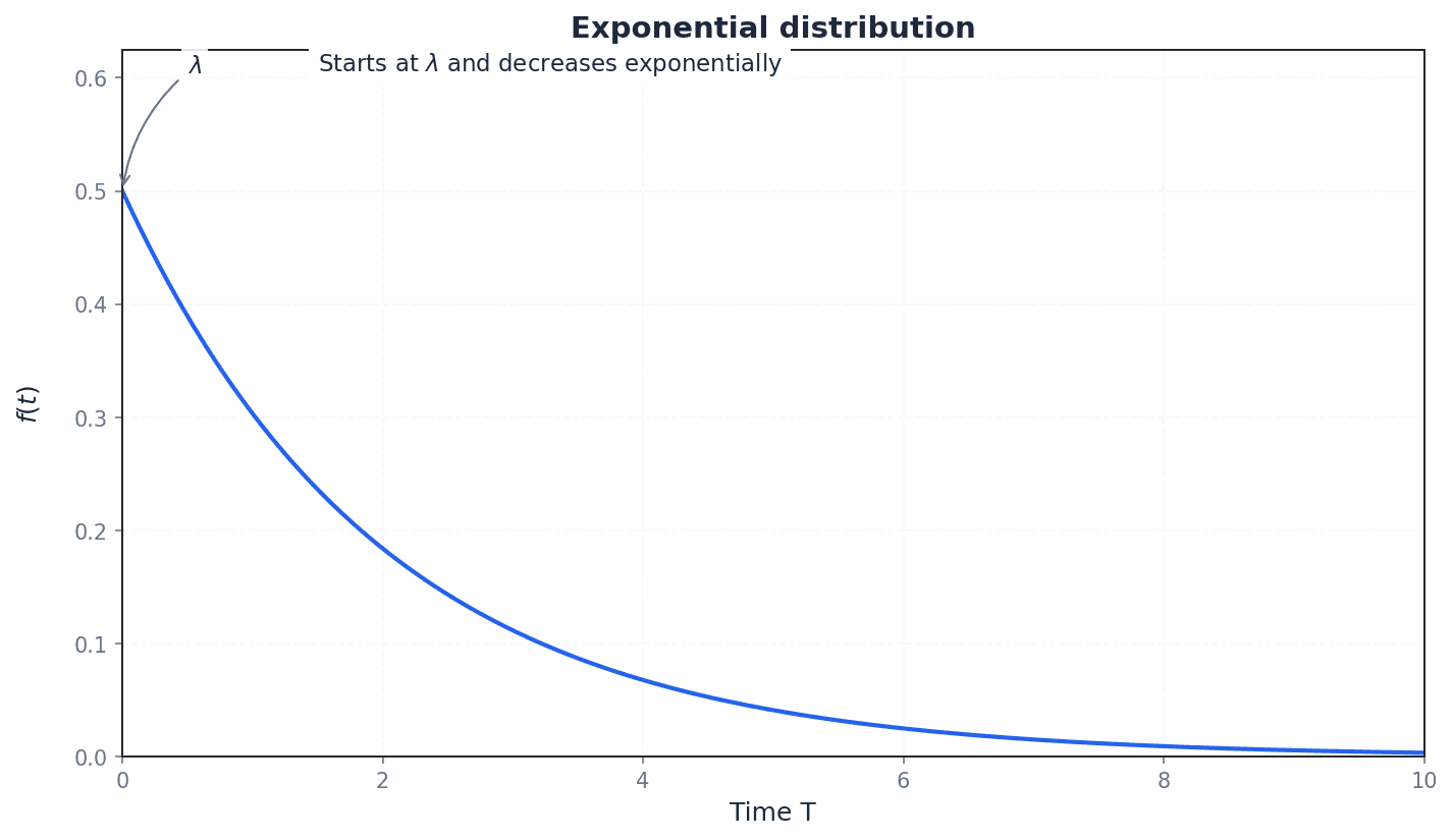
exponential distribution — A continuous random variable distribution where the probability density function is given by f(t) = λe^(-λt) for t ≥ 0, and 0 otherwise, where λ is a positive constant.
The exponential distribution models the time until some event occurs, particularly for events that happen continuously and independently at a constant average rate. It is characterized by a decreasing probability density as time increases. Think of the lifespan of a lightbulb that doesn't 'age' – it's just as likely to fail in the next hour whether it's new or has been on for a long time; the probability of it lasting longer decreases exponentially.
Properties of a Probability Density Function (PDF)
The probability density function cannot be negative.
Total Probability of all Outcomes
The total area under the graph of the PDF must equal 1.
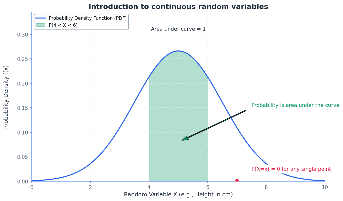
A continuous random variable can take any value within a given range, unlike discrete variables. Its probability distribution is described by a Probability Density Function (PDF), denoted f(x). For f(x) to be a valid PDF, it must satisfy two key properties: f(x) must be non-negative for all x, and the total area under its curve must integrate to 1. These properties ensure that the function correctly represents probability density.
Students often confuse the probability density f(x) with actual probability P(X=x). Remember that for a continuous random variable, the probability of any single exact value occurring is always zero, P(X=a) = 0. Only the area under the curve over an interval represents a probability.
When asked to 'show that f(x) has the properties of a probability density function', you must demonstrate two things: f(x) ≥ 0 for all x, and ∫f(x)dx = 1 over the entire range of the variable.
Probability of an Exact Value (Continuous Random Variable)
For a continuous random variable, the probability of any single exact value occurring is zero.
Probability within an Interval (Continuous Random Variable)
The probability of X lying in an interval is given by the area under the PDF graph between the bounds. The use of < or ≤ does not affect the probability.
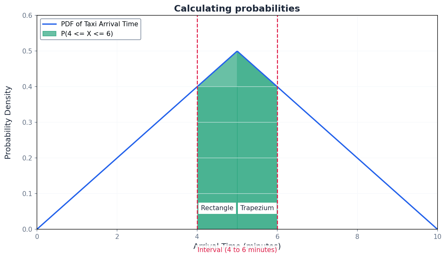
For continuous random variables, probabilities are not assigned to individual points but to intervals. The probability that a continuous random variable X falls within a certain interval [a, b] is found by integrating its PDF, f(x), over that interval. This integral represents the area under the curve of f(x) between a and b. It is important to note that for continuous variables, P(a < X < b) is equivalent to P(a ≤ X ≤ b), as the probability of X taking any exact value is zero.
Median of a Continuous Random Variable
The median is the value 'm' such that the area under the PDF from the lower limit to 'm' is 0.5.
The median (m) of a continuous distribution is the value that divides the total probability into two equal halves, meaning P(X ≤ m) = 0.5. It is calculated by integrating the PDF from its lower limit up to m and setting the result to 0.5, then solving for m. Similarly, any nth percentile (r) is found by setting the integral of the PDF from the lower limit to r equal to n/100, and solving for r.
Students often think the median is simply the middle value of the range. Actually, it's the value that splits the *probability* into two equal halves, which might not be the geometric center if the distribution is skewed.
When calculating the median or percentiles, ensure you integrate the correct part(s) of the PDF if it is defined piecewise, and always check that your calculated value falls within the domain of the function.
Expectation (Mean) of a Continuous Random Variable
Calculates the average value of the continuous random variable.
Expectation of X squared (for Variance)
Used as an intermediate step to calculate the variance of a continuous random variable.
Variance of a Continuous Random Variable
Calculates the spread of the distribution around the mean.
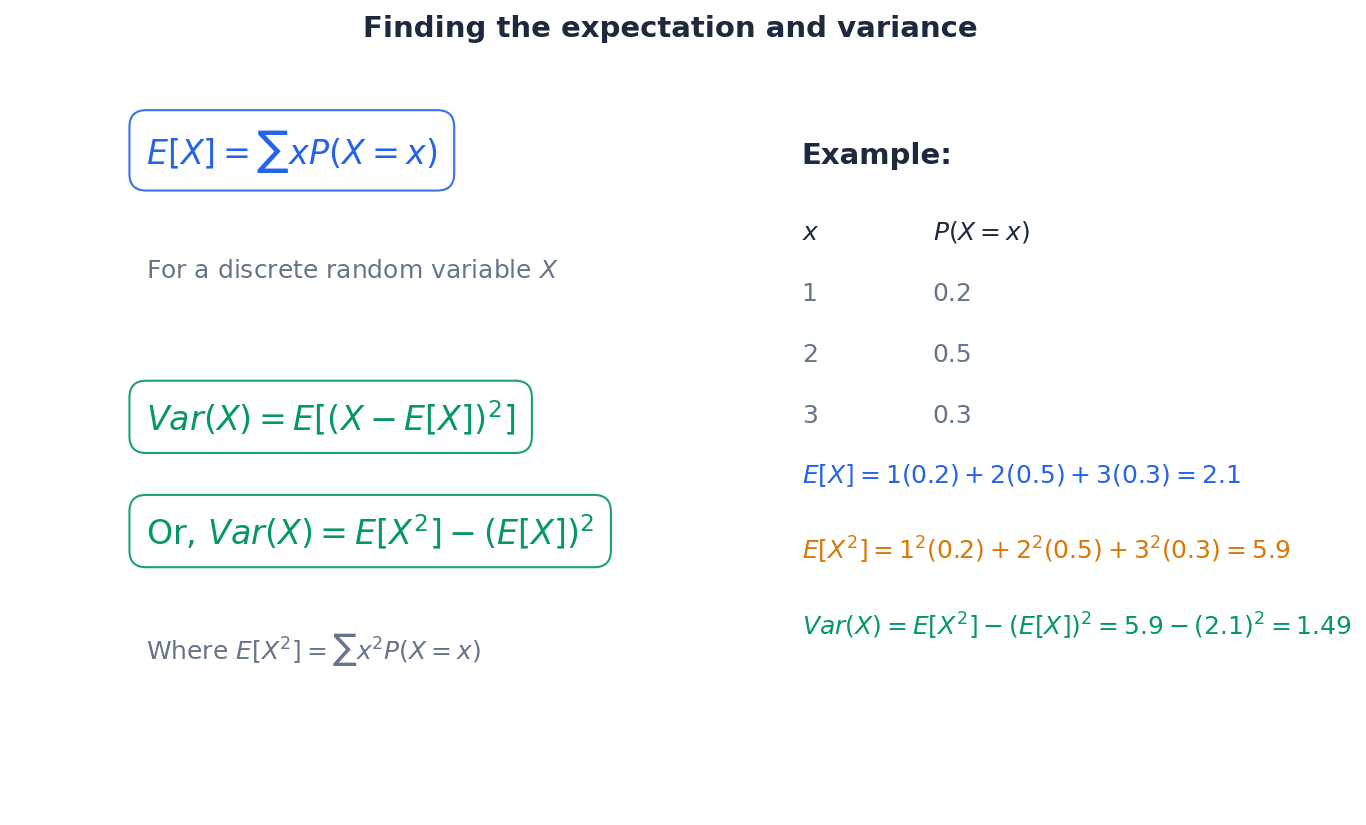
The expectation, or mean, E(X), of a continuous random variable X represents its average value. It is found by integrating the product of x and its PDF, f(x), over the entire range of the variable. The variance, Var(X), measures the spread of the distribution around the mean. It is calculated using the formula Var(X) = E(X^2) - (E(X))^2, where E(X^2) is found by integrating x^2 multiplied by the PDF over the entire range.
PDF of a Rectangular (Uniform) Distribution
Describes a distribution where all values within the interval [a, b] are equally likely.
Mean of a Rectangular (Uniform) Distribution
The mean is the midpoint of the interval for a uniform distribution.
Variance of a Rectangular (Uniform) Distribution
Formula for the variance of a uniform distribution over the interval [a, b].
A rectangular, or uniform, distribution is a specific type of continuous random variable where the probability density is constant across a defined interval [a, b] and zero elsewhere. This means every value within that interval has an equal chance of occurring. Its PDF is a horizontal line segment, and its mean is simply the midpoint of the interval, while its variance has a specific formula.
Students often think 'random' means uniform. However, a random variable can follow many distributions (e.g., normal, exponential), not just uniform.
PDF of an Exponential Distribution
Models the time until an event occurs, where events happen continuously and independently at a constant average rate.
Expectation (Mean) of an Exponential Distribution
The mean time until an event occurs in an exponential distribution.
Variance of an Exponential Distribution
The variance of the time until an event occurs in an exponential distribution.
The exponential distribution is used to model the time until an event occurs, particularly when events happen continuously and independently at a constant average rate. Its PDF is characterized by a decreasing probability density as time increases. For this distribution, the mean and variance have specific formulas related to the rate parameter λ, which can save time in calculations.
Students often confuse exponential distribution with normal distribution for 'time until event'. Remember that exponential distributions are memoryless and skewed, unlike the symmetrical normal distribution.
Always state the limits of integration clearly when calculating probabilities, mean, or variance. This is crucial for accuracy, especially with piecewise functions.
Be proficient with integration techniques, especially for expressions involving xf(x) and x²f(x) when calculating mean and variance. Practice these regularly.
When solving for median or percentiles from a quadratic equation, always select the root that falls within the defined domain of the PDF. Discard any extraneous solutions.
Exam Technique
Show that f(x) is a valid Probability Density Function (PDF)
Calculate the probability P(a < X < b)
| Mistake | Fix |
|---|---|
| Confusing probability density f(x) with actual probability P(X=x). | Remember that for continuous variables, P(X=x) is always zero. f(x) is a density, and only the area under the curve over an interval represents a probability. |
| Incorrectly assuming that the median is always the midpoint of the range of the variable. | The median is the value that splits the *probability* into two equal halves (P(X ≤ m) = 0.5), which might not be the geometric center if the distribution is skewed. Always calculate it using integration. |
| Making calculation errors when integrating piecewise functions for probabilities, median, mean, or variance. | Carefully split the integral into appropriate sections based on the function's definition and ensure correct limits of integration for each part. Double-check your integration steps and arithmetic. |
This chapter introduces the fundamental concepts of sampling, distinguishing between populations and samples, and explaining the necessity of random sampling to avoid bias. It explores the properties of sample means as random variables and culminates in the Central Limit Theorem, which allows us to approximate the distribution of sample means as normal for large sample sizes.
Population — The complete collection of items of interest.
This refers to the entire group that a study is interested in, whether it's people, objects, or events. For example, if you want to know the average height of all students in a school, the 'population' is every single student in that school. Decisions based on a whole population are often expensive and time-consuming to collect, process, and analyse.
Students often think 'population' only refers to people, but actually it can be any complete collection of items, like fish, buttons, or LED lights. Remember to specify 'complete collection of items of interest' in definitions.
Sample — A part of a population.
A sample is a subset of the population from which data is collected. It is used to test theories or hypothesise about the larger population, especially when collecting data from the entire population is impractical or impossible. For instance, if you taste a spoonful of soup to check its seasoning, that spoonful is a 'sample' of the entire pot of soup.
Sampling frame — The complete list of all items or people in the population.
This list is essential for generating a truly random sample, as it allows every member of the population to be assigned a number and thus have an equal chance of selection. Without a complete sampling frame, some members cannot be selected, leading to selection bias. A school's official register of all enrolled students would serve as a sampling frame if you wanted to randomly select students from that school.
Students often think a sampling frame is just any list, but actually it must be a *complete* list of the *entire* population to avoid selection bias.
Random sample — A random sample of size n is a sample selected in such a way that all possible samples of size n that you could select from the population have the same chance of being chosen.
This is the most basic sampling technique, ensuring every member of the population has an equal chance of selection. It requires a complete list of the population, known as the sampling frame, which may not always be available. Drawing names out of a hat where every name is written on an identical slip of paper and mixed thoroughly is an example of creating a random sample.
When describing random sampling, ensure you mention the equal chance of selection for every member and the need for a complete sampling frame.
Random numbers — Values generated entirely by chance, used to select a random sample.
Random numbers ensure that the selection process is unbiased, giving every member of the population an equal chance of being chosen. They can be generated using tables, calculators (RAND/RND/RAN# functions), or computational random number generators. This is like drawing lottery numbers, where each number has an equal chance of being picked, to select items from a list without any pattern or preference.
When asked to describe using random numbers for sampling, detail the steps: numbering the population, choosing a starting point, and handling repeats or numbers outside the range.
Students often think that picking numbers 'at random' by hand is sufficient, but actually true random numbers require a systematic method to avoid human bias.
Biased — A sampling technique that results in an unrepresentative sample is said to be biased.
Bias occurs when one or more characteristics of a population are over- or under-represented in the sample, favouring certain parts of the population over others. This makes the sample unrepresentative and can lead to invalid conclusions. For example, if you want to know what people think of a new chocolate bar and only ask people who have just bought it, your sample will be biased towards those who already like it.
When asked to identify bias, explain *why* the method leads to an unrepresentative sample, not just that it is biased. Suggest ways to avoid it.
Students often think bias only comes from intentional manipulation, but actually selection bias can be unintentional, arising from how the sample is chosen.
Sample size — The number of items you choose to be in your sample.
The sample size, denoted by 'n', is a crucial factor affecting the reliability and representativeness of a sample. A larger sample size generally leads to more reliable conclusions, especially when applying the Central Limit Theorem. For instance, if you're baking a cake and taste a small crumb, that's a small sample size. Tasting a larger slice gives you a better idea of the whole cake's flavour, representing a larger sample size.
Students often think a larger sample is always better, but actually a reasonably large sample chosen randomly is generally representative, and excessively large samples can be inefficient.
Sampling is studied because collecting data from an entire population is often impractical, impossible, or too expensive and time-consuming. By taking a representative sample, we can make inferences and test theories about the larger population without needing to examine every single item. The reliability of these inferences depends heavily on how the sample is chosen and its size.
Sample mean — The mean of all the items in your chosen sample.
The sample mean is a statistic calculated from a sample, used as an estimate for the population mean. Different samples from the same population will likely have different sample means, and these means themselves form a distribution. If you measure the heights of 10 students from a class, the average of those 10 heights is the sample mean.
Students often think the sample mean will always be exactly equal to the population mean, but actually it's an estimate and will vary from sample to sample. Distinguish clearly between the sample mean (X̄) and the population mean (µ).
Mean of sample means
This formula applies when a random sample consists of n observations of a random variable X. It states that the expected value of the sample mean is equal to the population mean.
Variance of sample means
This formula applies when a random sample consists of n observations of a random variable X. It shows that the variance of the sample mean decreases as the sample size (n) increases.
The sample mean (X̄) can be regarded as a random variable itself, as its value will vary from one sample to another. If the original population X has a normal distribution, then the distribution of the sample mean X̄ will also be normal, with mean µ and variance σ²/n. This property is crucial for making probability statements about sample means when the population is known to be normal.
Central limit theorem — For large sample sizes, the distribution of a sample mean is approximately normal, regardless of whether the underlying population is normal.
This fundamental theorem states that if you take many random samples of size 'n' from any population with mean µ and variance σ², the distribution of these sample means (X̄) will be approximately normal with mean µ and variance σ²/n, provided 'n' is sufficiently large. This allows the use of normal distribution for statistical judgments from sample data from any distribution. Imagine you have a bag of oddly shaped, weighted dice; if you roll one die many times and average the results, the average will tend towards a normal distribution, even though the individual die rolls are not normally distributed.
Distribution of sample means (Central Limit Theorem)
This applies when n is large (typically n ≥ 30 for any population, or lower if the original population is approximately normal). It describes the approximate normal distribution of the sample mean.
When applying the Central Limit Theorem, explicitly state that 'n is large' and specify the parameters of the resulting normal distribution (mean µ and variance σ²/n).
Students often think the Central Limit Theorem means the *original population* becomes normal, but actually it's the *distribution of sample means* that becomes approximately normal. Also, remember that the required 'largeness' of the sample size depends on the original population's distribution.
Always state the distribution you are using for X̄ (e.g., X̄ ~ N(μ, σ²/n)) before performing calculations.
Show clear working for calculating probabilities involving sample means, including standardising to Z-scores. Pay attention to whether the question refers to the distribution of the population or the distribution of the sample mean.
Exam Technique
Calculating mean and variance of sample means
Finding probabilities for sample means (population normally distributed)
| Mistake | Fix |
|---|---|
| Confusing population parameters with sample statistics. | Clearly distinguish between µ (population mean) and X̄ (sample mean), and σ² (population variance) and Var(X̄) = σ²/n (variance of sample mean). |
| Forgetting to divide the population variance by 'n' when calculating the variance of the sample mean. | Always remember the formula Var(X̄) = σ²/n. The variance of the sample mean is smaller than the population variance. |
| Applying the Central Limit Theorem without stating the condition 'n is large'. | Explicitly state 'n is large, so by the Central Limit Theorem...' before using X̄ ~ N(µ, σ²/n). |
This chapter focuses on estimation, teaching how to use sample data to make inferences about unknown population parameters. It covers calculating unbiased estimates for population mean and variance, performing hypothesis tests for the population mean, and constructing confidence intervals for population means and proportions. The precision and reliability of these estimates are heavily influenced by sample size and confidence level.
Population — Refers to the complete collection of items in which you are interested.
This is the entire group of individuals or objects that a researcher wants to draw conclusions about. It is often too large to study directly, so samples are taken to represent it.
Sample — A part of a population.
A sample is a subset of the population that is selected for study. Information from the sample is used to make inferences about the entire population. For example, if you want to know the average height of all students in a country, measuring the heights of 100 students from different schools would be your sample.
Parameter — A value that summarises data for a population.
Parameters are fixed, unknown values that describe characteristics of an entire population, such as the population mean (µ) or population variance (σ²). They are estimated using statistics calculated from samples, like the true average height of all adults in a country.
Statistic (also known as an estimate) — A numerical value calculated from a set of data and used in place of an unknown parameter in a population.
A statistic is a value derived from a sample, such as the sample mean (¯x) or sample variance (s²), which serves as an estimate for an unknown population parameter. For instance, if you measure the heights of 10 friends and calculate their average, that's a sample mean for your group of friends.
Students often confuse population parameters (µ, σ²) with sample statistics (¯x, s²). Remember that parameters describe populations (fixed, unknown), while statistics describe samples (variable, known).
Random sampling — Means that every possible sample of a given size is equally likely to be chosen.
A random sample of size n is selected so that all possible samples of that size from the population have the same chance of being chosen. This helps ensure the sample is representative and reduces bias, much like drawing names out of a hat where every name has an equal chance of being picked.
Sampling frame — A list of the whole population.
This is a complete and accurate list of all the units in the population from which a sample can be drawn. It is essential for implementing random sampling methods, for example, a school's student roster if you want to sample students from that school.
Bias — Bias is the tendency of a statistic to overestimate or underestimate a parameter.
An estimate is biased if its expected value is not equal to the true value of the population parameter it is estimating. This difference is known as sampling error. For example, if you always guess a person's age to be higher than it actually is, your guesses are biased upwards.
Unbiased estimate — A statistic is an unbiased estimate of a given population parameter when the mean of the sampling distribution of that statistic is equal to the parameter being estimated.
An unbiased estimate, on average, will hit the true population parameter. This is a desirable property for an estimator, ensuring that there is no systematic over or underestimation.
Sampling error — The error from choosing an unrepresentative sample.
This is the natural variability that occurs when a sample is used to estimate a population parameter. It is the difference between the expected value of an estimate and the true value of the parameter, often due to chance. For instance, if you randomly pick 10 marbles from a bag of 100 (50 red, 50 blue) and happen to get 7 red, the difference from the expected 5 red is sampling error.
Selection bias — The unintentional selection of one group or outcome of a population over potential other groups or outcomes of the population.
This occurs when the sample selection method systematically favors certain individuals or groups, leading to a sample that is not representative of the population. It can lead to inaccurate conclusions, such as only surveying people at a gym about their exercise habits, which would give a biased view of the general population's exercise habits.
When we collect data from a sample, our goal is often to estimate unknown characteristics of the larger population. The sample mean (¯x) is an unbiased estimate for the population mean (µ), meaning that, on average, sample means will equal the population mean. For the population variance (σ²), a specific formula is used to ensure the estimate is unbiased, which involves dividing by (n-1) rather than n.
Unbiased estimate for population mean
Used for sample size n taken from a population.
Unbiased estimate for population variance (raw data)
Used for raw data. Also written as s^2 = \frac{1}{n-1} (\sum x^2 - n\bar{x}^2).
Unbiased estimate for population variance (summarised data)
Used for summarised data. On calculators, this corresponds to s_{n-1} or σ_{n-1}.
Students often forget to use (n-1) in the denominator when calculating the unbiased estimate of population variance. Remember this is crucial for an unbiased estimate.
When asked to explain bias, refer to the expected value of the estimate not equalling the true parameter, rather than just stating it over/underestimates.
Random variable — Describes the numerical outcomes of a situation.
A random variable is a variable whose value is a numerical outcome of a random phenomenon. It can be discrete (countable outcomes) or continuous (measurable outcomes). For example, the number of heads in 3 coin flips is a random variable, as its value (0, 1, 2, or 3) depends on a random event.
Discrete random variable — Has outcomes that are countable distinct values.
Unlike continuous variables, discrete variables can only take on specific, separate values, often integers. Probabilities are associated with each distinct value, such as the number of heads when flipping a coin 5 times.
Continuous random variable — The outcome of a continuous random variable can take an infinite number of possible values; these are usually measurements.
Unlike discrete variables, continuous variables can take any value within a given range. Probabilities are associated with intervals rather than specific points, and are described by a probability density function. The height of a person or the time it takes to run a race are continuous random variables.
Probability distribution — Describes the probabilities associated with each possible value of a discrete random variable.
This can be presented as a table, graph, or formula, showing all possible outcomes of a discrete random variable and their corresponding probabilities. The sum of all probabilities must equal 1. For example, a list of all possible scores you can get on a die (1, 2, 3, 4, 5, 6) and the probability of rolling each one (1/6 for each) is a probability distribution.
Probability density function (PDF) — A function that describes the probabilities of a continuous random variable; its graph is never negative.
For a continuous random variable, the area under the PDF curve between two points gives the probability that the variable falls within that range. The total area under the curve must equal 1. Imagine a landscape where the height of the land represents the PDF; the probability of finding yourself in a certain region is proportional to the 'amount of land' (area) in that region.
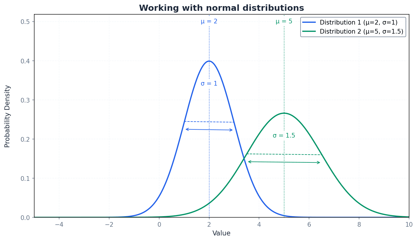
Normal distribution — A continuous random distribution used to describe many naturally occurring phenomena.
It is characterized by its bell-shaped curve and is symmetrical around its mean. It is widely used in statistics due to the Central Limit Theorem and its mathematical properties, allowing for approximations of other distributions. The distribution of human heights or IQ scores often approximates a normal distribution.
Binomial distribution — A discrete distribution where there is a fixed number, n, of trials with only two outcomes, success or failure, where the probability of success is p.
This distribution models the number of successes in a fixed number of independent Bernoulli trials. It is often approximated by a normal distribution for large n, or a Poisson distribution for large n and small p. Flipping a coin 10 times and counting the number of heads follows a binomial distribution.
Poisson distribution — A discrete distribution where the number of occurrences of an event occur independently, at random and at a constant average rate.
This distribution models the number of events occurring in a fixed interval of time or space. It is characterized by a single parameter, λ (lambda), which represents both its mean and variance. The number of phone calls received by a call center in an hour can often be modeled by a Poisson distribution.
Central limit theorem — States that, provided n is large, the distribution of sample means of size n is X ~ N(µ, σ²/n) where the original population has mean µ and variance σ².
This theorem is fundamental because it allows the use of the normal distribution for statistical inference about population means, even if the original population distribution is not normal, provided the sample size is sufficiently large. It explains why sample means tend to be normally distributed, like how the average size of pebbles in many handfuls will tend to follow a normal distribution, even if the pebbles in the pile aren't normally distributed.
Students often think the Central Limit Theorem means the original population is normal, but actually it applies to the distribution of sample means, regardless of the original population's distribution (for large n).
When using the Central Limit Theorem, explicitly state that 'n is large' as an assumption, and remember to use σ²/n for the variance of the sample mean.
Hypothesis testing is a formal procedure to investigate if a claim about a population parameter could happen by chance or if the probability of it occurring by chance is statistically significant. It involves setting up a null hypothesis (H0) and an alternative hypothesis (H1), calculating a test statistic, and comparing it to critical values to make a decision. This process helps determine if there is enough evidence to reject the initial assumption (H0).
Hypothesis — A claim believed or suspected to be true.
In statistics, a hypothesis is a statement about a population parameter that is subject to testing using sample data. It forms the basis for statistical inference, similar to a detective's initial 'hunch' about a case that needs to be investigated.
Null hypothesis, H0 — The assumption that there is no difference between the parameter being tested and the sample data.
This is the default assumption in a hypothesis test, often stating no effect, no difference, or no change. The goal of the test is to determine if there is sufficient evidence to reject this hypothesis in favor of the alternative hypothesis. For example, in a drug trial, the null hypothesis is that the new drug has no effect compared to a placebo.
Students often state H0 as 'the sample mean is equal to X', but actually H0 should always be about the population parameter (e.g., 'the population mean is equal to X').
Alternative hypothesis, H1 — The hypothesis that the observations being considered in a hypothesis test are influenced by some non-random cause; the abbreviation for the alternative hypothesis is H1.
This is the hypothesis that contradicts the null hypothesis and is accepted if the null hypothesis is rejected. It typically represents the claim or effect that the researcher is trying to find evidence for. If the null hypothesis is 'the coin is fair', the alternative hypothesis might be 'the coin is biased'.
Ensure H1 is stated correctly as a one-tailed or two-tailed test based on the wording of the problem, as this affects the critical region.
Hypothesis test — The investigation to find out if a claim could happen by chance or if the probability of it occurring by chance is statistically significant.
This is a formal procedure for making decisions about population parameters based on sample data. It involves setting up null and alternative hypotheses, calculating a test statistic, and comparing it to critical values or p-values. It's like a court trial: the null hypothesis is 'innocent until proven guilty', and the test determines if there's enough evidence to reject 'innocent'.
Significance level — The percentage level at which the null hypothesis is rejected.
Commonly denoted by α, it is the probability of making a Type I error (rejecting a true null hypothesis). Typical values are 5% (0.05) or 1% (0.01). It defines the critical region, much like the 'burden of proof' in a court case.
Students often confuse the significance level with the p-value, but actually the significance level is set *before* the test, while the p-value is calculated *from* the data.
Test statistic — The calculated value in a hypothesis test.
This is a value calculated from the sample data during a hypothesis test. Its magnitude and sign indicate how far the sample result deviates from what would be expected under the null hypothesis. This value is then compared to critical values to make a decision.
Critical value — The boundary of the critical region.
This is the threshold value(s) from the sampling distribution that determines whether the test statistic falls into the critical region or the acceptance region. It is determined by the significance level and the type of test (one-tailed or two-tailed). It's like the 'pass/fail' score on an exam.
Students often confuse the critical value with the test statistic, but actually the critical value is a fixed boundary determined by the significance level, while the test statistic is calculated from the sample data.
Critical region (or rejection region) — The area of a graph, or set of values, for which you reject the null hypothesis.
If the calculated test statistic falls into this region, the result is considered statistically significant, leading to the rejection of the null hypothesis. The boundary of this region is defined by the critical value(s). In a game of 'hot or cold', the critical region is the 'hot' zone where the evidence is strong enough to say something unusual is happening.
Rejection region — See critical region.
This is an alternative term for the critical region, emphasizing that if the test statistic falls within this area, the null hypothesis is rejected. It's the 'danger zone' for the null hypothesis; if your data lands here, the null hypothesis is in trouble.
Acceptance region — The area of the graph, or set of values, for which you accept the null hypothesis.
In hypothesis testing, if the calculated test statistic falls within this region, there is insufficient evidence to reject the null hypothesis. It represents the range of outcomes considered consistent with the null hypothesis. Imagine a target in archery; the acceptance region is the bullseye and inner rings where your shot is considered 'good enough' to confirm your aim.
One-tailed hypothesis test — In this test, the alternative hypothesis looks for an increase or decrease in the parameter.
The critical region for a one-tailed test is located entirely in one tail of the sampling distribution (either upper or lower), reflecting a directional hypothesis. This is used when there is a specific expectation about the direction of the effect, such as testing if a new fertilizer *increases* crop yield.
Students often use a one-tailed test when the question asks 'is there a difference?', but actually 'difference' implies a two-tailed test unless a specific direction is stated.
Two-tailed hypothesis test — In this test, the alternative hypothesis looks for a difference from the parameter.
A two-tailed test is used when the alternative hypothesis states that the population parameter is simply 'not equal to' the hypothesized value, without specifying a direction. The critical region is split between both tails of the sampling distribution.
Type I error — A Type I error is said to have occurred when a true null hypothesis is rejected.
This is also known as a false positive. The probability of making a Type I error is equal to the significance level (α) set for the test. For example, concluding a drug has an effect when it actually doesn't.
Type II error — A Type II error is said to have occurred when a false null hypothesis is accepted.
This is also known as a false negative. It means failing to detect an effect that actually exists. For example, concluding a drug has no effect when it actually does.
Standard error — The standard deviation of sample mean, σ/√n.
It measures the variability of sample means around the true population mean. A smaller standard error indicates that sample means are more tightly clustered around the population mean, leading to more precise estimates. If you repeatedly weigh a bag of apples, the standard error tells you how much your average weight measurements are likely to vary from the true average weight of all apples.
Students often confuse standard error with standard deviation, but actually standard deviation describes the spread of individual data points, while standard error describes the spread of sample means.
Test statistic for population mean (known variance)
Used when the population is normally distributed with known variance, or for a large sample size (due to Central Limit Theorem).
Test statistic for population mean (unknown variance, large sample)
Used for a large sample size (n ≥ 30) when the population variance is unknown. Here, s is the unbiased estimate of the population standard deviation.
Always conclude a hypothesis test in the context of the original problem, clearly stating whether H0 is rejected or not and what this implies.
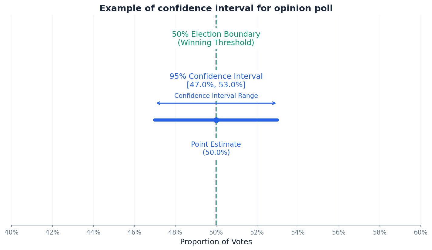
A confidence interval provides a range of values, calculated from sample data, that is likely to contain the true population parameter with a certain level of confidence (e.g., 95%). It quantifies the uncertainty associated with an estimate, offering a more informative picture than a single point estimate. The width of the interval is influenced by the confidence level and the sample size.
Confidence interval (CI) — An interval that specifies the limits within which it is likely that the population mean will lie.
A confidence interval provides a range of values, calculated from sample data, that is likely to contain the true population parameter with a certain level of confidence (e.g., 95%). It quantifies the uncertainty associated with an estimate. If you're trying to guess the average height of all students in a school, a confidence interval is like saying 'I'm 95% sure the average height is between 160 cm and 170 cm', rather than giving a single guess.
Students often think a 95% confidence interval means there's a 95% chance the true mean is in *this specific interval*, but actually it means that if you repeat the sampling many times, 95% of the intervals constructed would contain the true mean.
Confidence interval for population mean (known variance)
Used when the population is normally distributed with known variance. The interval is (\bar{x} - k \frac{\sigma}{\sqrt{n}}, \bar{x} + k \frac{\sigma}{\sqrt{n}}).
Confidence interval for population mean (large sample, unknown variance)
Used for a large sample size (n ≥ 30) when the population variance is unknown. The interval is (\bar{x} - k \frac{s}{\sqrt{n}}, \bar{x} + k \frac{s}{\sqrt{n}}).
Always interpret a confidence interval in context, stating the confidence level and what parameter the interval estimates. Be precise about what the interval represents.
When dealing with categorical data, we often want to estimate the proportion of a population that possesses a certain characteristic. For a large random sample, the binomial distribution, which models proportions, can be approximated by a normal distribution. This allows us to construct an approximate confidence interval for the population proportion, providing a range within which the true proportion is likely to lie.
Confidence interval for population proportion (large sample)
Used for a large random sample where np > 5 and n(1-p) > 5. This is an approximate confidence interval.
Always clearly state your hypotheses (H₀ and H₁) and the significance level (α) at the start of a hypothesis test.
Show all steps in hypothesis testing: calculate test statistic, find critical value/p-value, compare, and state your conclusion in context.
When constructing confidence intervals, clearly state the formula used and substitute values correctly, showing the final interval.
Exam Technique
Calculate unbiased estimates of population mean and variance
Carry out a hypothesis test for population mean
| Mistake | Fix |
|---|---|
| Confusing population parameters (µ, σ²) with sample statistics (¯x, s²). | Always use Greek letters for population parameters and Roman letters for sample statistics. Remember parameters are fixed but unknown, statistics are calculated from samples and vary. |
| Assuming a sample mean is the true population mean. | The sample mean is an *estimate* of the population mean. It will vary from sample to sample due to sampling error. A confidence interval provides a range for the true mean. |
| Misinterpreting the meaning of a confidence interval. | A 95% CI means that if you repeat the sampling process many times, 95% of the intervals constructed would contain the true mean. It does NOT mean there's a 95% chance the true mean is in *this specific* interval. |
Generated by Nexelia Academy · nexeliaacademy.com