Nexelia Academy · Official Revision Notes
Complete A-Level revision notes · 9 chapters
This chapter explores quadratic equations and functions, covering various methods for solving them, including factorisation, completing the square, and the quadratic formula. It also delves into quadratic inequalities, simultaneous equations involving quadratics, and understanding the graphical properties of quadratic functions.
parabola — The shape of the graph of a quadratic function f(x) = ax^2 + bx + c.
A parabola is a symmetrical curve that opens either upwards (if a > 0) or downwards (if a < 0). It has a single turning point called the vertex, which is either a maximum or minimum. Imagine the path a ball takes when thrown through the air; this trajectory is a parabola.
vertex — The maximum or minimum point of a parabola.
The vertex is the turning point of the parabola, where the gradient is zero. It lies on the line of symmetry of the parabola and represents the extreme value (maximum or minimum) of the quadratic function. Think of the peak of a mountain or the bottom of a valley; the vertex is the highest or lowest point on the curve.
stationary point — A point where the gradient of a curve is zero.
For a quadratic function, the stationary point is always the vertex, which is either a maximum or minimum. More generally, for other functions, stationary points can also be points of inflection. Imagine a car momentarily stopping at the top of a hill or the bottom of a dip; at that exact moment, its vertical speed (gradient) is zero.
Students often think a stationary point is always a turning point, but actually it can also be a point of inflection where the curve changes concavity without turning.
turning point — A point where the gradient of a curve is zero and the curve changes direction (from increasing to decreasing or vice versa).
For a quadratic function, the turning point is the vertex, which is either a maximum or minimum. It is where the function reaches its extreme value. Similar to a stationary point, it's where a roller coaster reaches its highest or lowest point before changing direction.
Students often confuse turning points with x-intercepts, but actually turning points relate to the maximum/minimum value of the function, not where it crosses the x-axis.
roots — The solutions to the equation f(x) = 0 for a function f(x).
For a quadratic equation ax^2 + bx + c = 0, the roots are the values of x that satisfy the equation. Graphically, these are the x-coordinates where the curve y = f(x) intersects the x-axis. Think of the roots of a tree; they are the fundamental points where the tree connects to the ground, just as the roots of an equation are the fundamental x-values where the graph touches the x-axis.
Students often confuse roots with the vertex, but actually roots are where the graph crosses the x-axis, while the vertex is the maximum or minimum point of the curve.
Quadratic Formula
Used to solve quadratic equations of the form ax^2 + bx + c = 0.
Discriminant
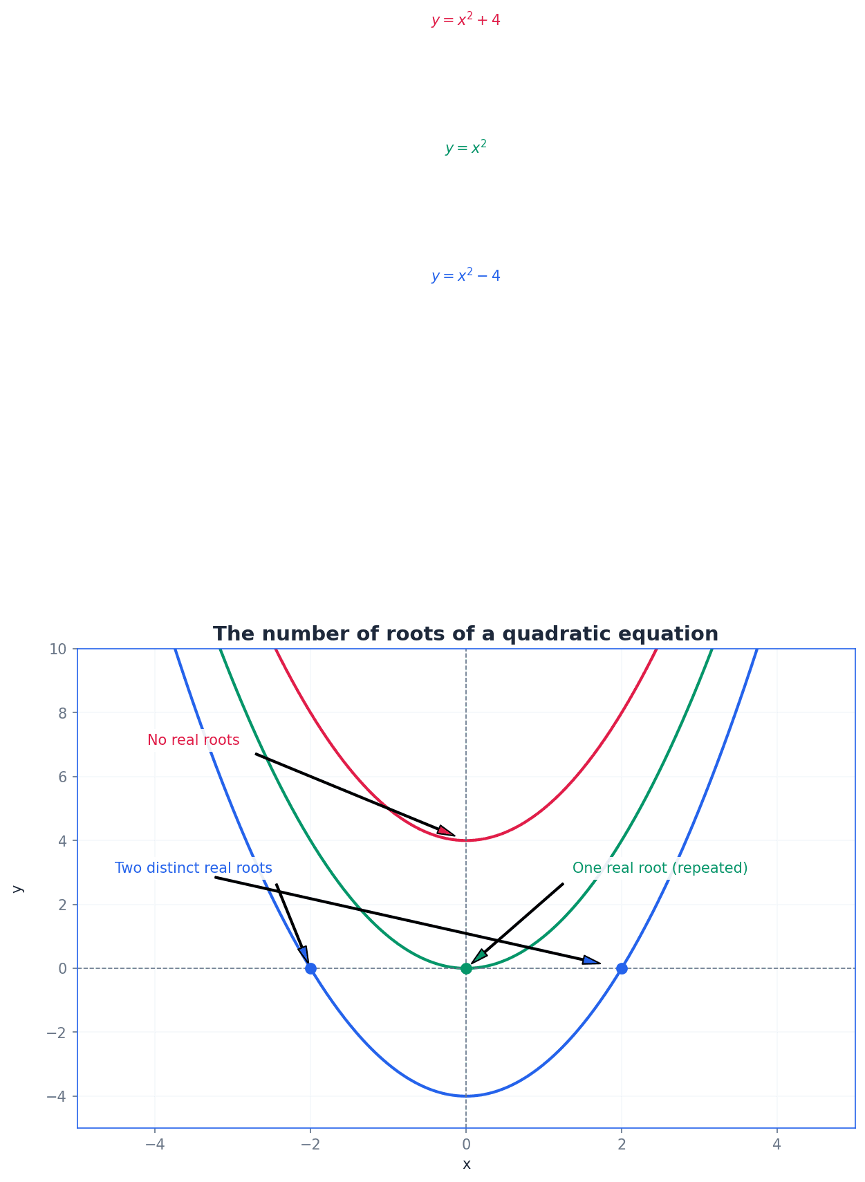
Determines the nature of the roots of a quadratic equation ax^2 + bx + c = 0. If Δ > 0, two distinct real roots; if Δ = 0, two equal real roots; if Δ < 0, no real roots.
discriminant — The part of the quadratic formula underneath the square root sign, b^2 - 4ac.
The sign of the discriminant (positive, zero, or negative) determines the nature and number of real roots of a quadratic equation. It indicates whether there are two distinct real roots, two equal real roots, or no real roots. Consider the discriminant as a 'root detector' for quadratic equations; it tells you what kind of roots to expect without fully solving the equation.
Students often forget to consider the case where a=0 when using the discriminant, but actually the discriminant only applies to quadratic equations (where a ≠ 0).
two distinct real roots — A condition for a quadratic equation where the discriminant is positive (b^2 - 4ac > 0), resulting in two different real number solutions.
Graphically, this means the parabola intersects the x-axis at two separate points. Algebraically, the quadratic formula will yield two different real values for x. Imagine a river splitting into two separate streams; each stream represents a distinct real root.
Students often confuse 'two distinct real roots' (b^2 - 4ac > 0) with 'real roots' (b^2 - 4ac ≥ 0), but actually 'distinct' specifically means the two roots are different values.
two equal real roots — A condition for a quadratic equation where the discriminant is zero (b^2 - 4ac = 0), resulting in exactly one real number solution (a repeated root).
Graphically, this means the parabola touches the x-axis at exactly one point, which is its vertex. Algebraically, the quadratic formula yields the same real value for x twice. Think of a car just touching a speed bump at its highest point; it makes contact at only one specific spot.
Students often think 'two equal roots' means no roots, but actually it means there is one unique real root that appears twice in the solution set.
no real roots — A condition for a quadratic equation where the discriminant is negative (b^2 - 4ac < 0), meaning there are no real number solutions.
Graphically, this means the parabola does not intersect the x-axis at all; it is either entirely above or entirely below the x-axis. Algebraically, taking the square root of a negative number results in imaginary solutions, not real ones. Imagine a bridge that never touches the water below; it exists entirely above the surface, just as a curve with no real roots exists entirely above or below the x-axis.
Students often think 'no real roots' means no solutions at all, but actually it means no solutions within the set of real numbers; there are still complex (non-real) solutions.
Quadratic equations, in the form ax^2 + bx + c = 0, can be solved using several methods. Factorisation is often the quickest if possible, by expressing the quadratic as a product of linear factors. If factorisation is not straightforward, completing the square or using the quadratic formula are reliable alternatives. The quadratic formula is universally applicable for any quadratic equation.
Always check if factorisation is possible before resorting to the quadratic formula or completing the square.
Completing the square is a method to transform a quadratic polynomial ax^2 + bx + c into the form a(x+p)^2 + q. This form is particularly useful for identifying the vertex of the parabola and solving equations that are not easily factorised. The vertex of the parabola is given by (-p, q).
When completing the square, ensure you correctly handle the coefficient 'a' if it's not 1.
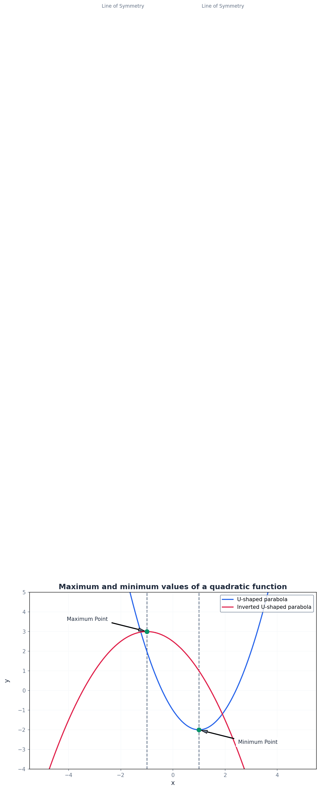
line of symmetry — A vertical line that passes through the vertex of a parabola, dividing it into two mirror-image halves.
For a quadratic function f(x) = a(x-h)^2 + k, the line of symmetry is x = h. For f(x) = ax^2 + bx + c, the line of symmetry is x = -b/(2a). Think of folding a piece of paper in half so that both sides match perfectly; the fold line is the line of symmetry.
Students often confuse the line of symmetry with the x-axis, but actually the line of symmetry is a vertical line passing through the vertex, not necessarily the x-axis.
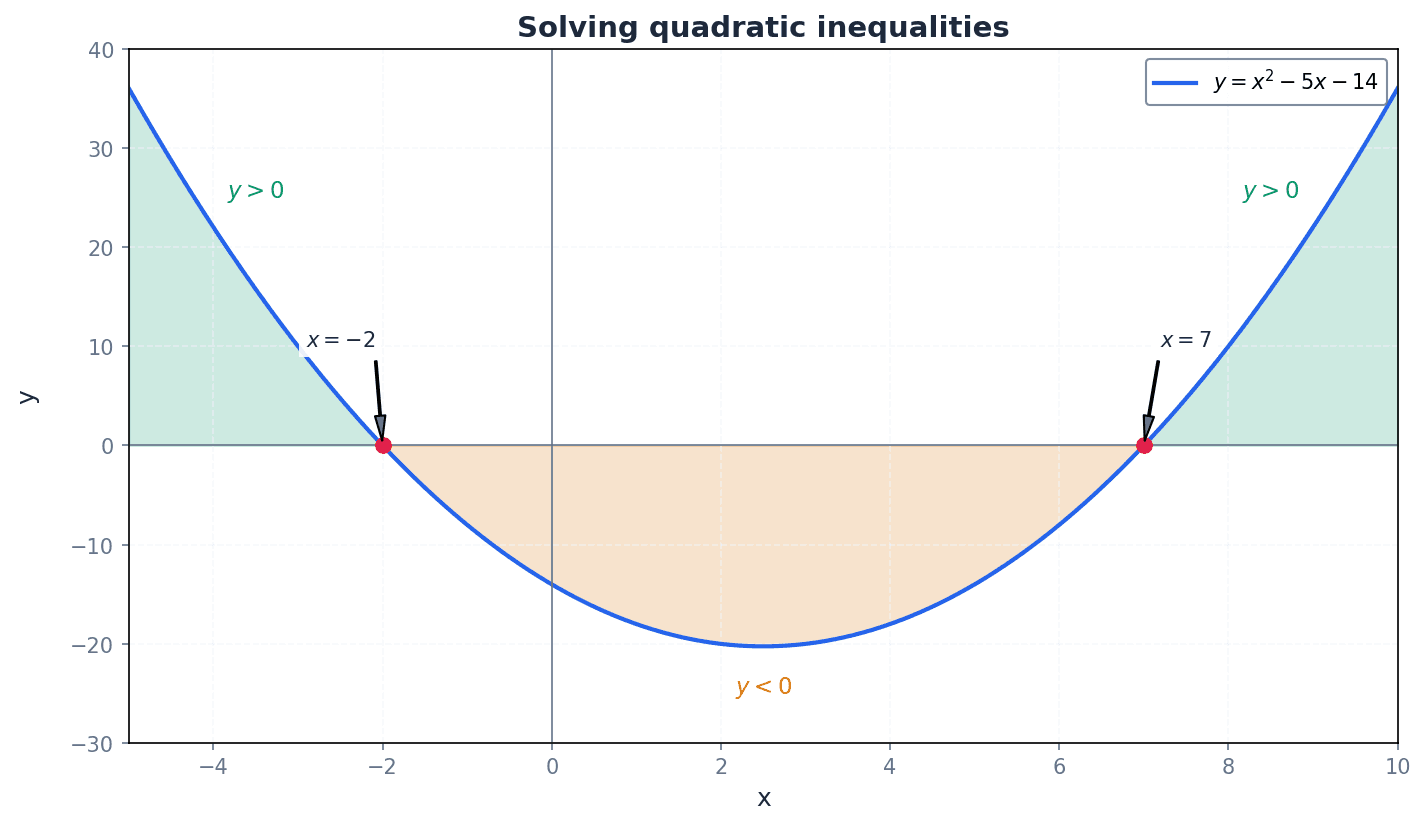
Solving quadratic inequalities involves finding the range of x-values for which a quadratic expression is greater than or less than zero. This typically involves finding the roots of the associated quadratic equation (critical values) and then using a sketch of the parabola to determine the regions that satisfy the inequality.
curve is positive — The range of x-values for which the y-values of a function are greater than zero (y > 0).
Graphically, this corresponds to the parts of the curve that lie above the x-axis. When solving inequalities like f(x) > 0, you are looking for these regions. Imagine a roller coaster track; the parts of the track that are above ground level represent where the curve is positive.
Students often confuse 'curve is positive' with 'positive gradient', but actually 'curve is positive' refers to the y-value being positive, while 'positive gradient' refers to the slope of the curve.
For quadratic inequalities, sketching the parabola helps visualise the solution set and avoid errors.
Students often forget to reverse the inequality sign when multiplying or dividing both sides of an inequality by a negative number.
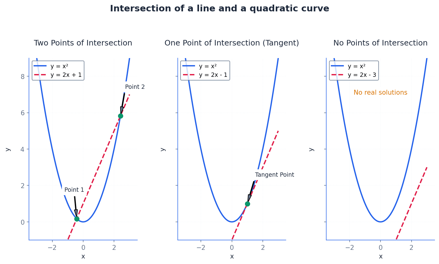
To find the points of intersection between a linear equation and a quadratic equation, substitute the linear equation into the quadratic one. This results in a single quadratic equation in one variable, which can then be solved. The solutions for x are the x-coordinates of the intersection points, and these must be substituted back into the linear equation to find the corresponding y-coordinates.
points of intersection — The coordinates where two or more graphs meet.
For a line and a quadratic curve, these points are found by solving their equations simultaneously. The number of real solutions corresponds to the number of points of intersection. Imagine two roads crossing each other; the points where they cross are the points of intersection.
Students often only find the x-coordinates when solving simultaneous equations for points of intersection, forgetting to find the corresponding y-coordinates.
When solving simultaneous equations, substitute the linear equation into the quadratic one to form a single quadratic equation.
When asked for a 'turning point', ensure you provide both the x and y coordinates. Completing the square is an efficient method to find the coordinates of the turning point for a quadratic.
Always verify your solutions by substituting them back into the original equations, especially for simultaneous equations.
Exam Technique
Solving quadratic equations by factorisation
Completing the square for ax^2 + bx + c
| Mistake | Fix |
|---|---|
| Incorrectly dividing by a variable (e.g., x) when solving equations. | Always factorise out common variables instead of dividing, to avoid losing valid solutions (e.g., in 3x^2 + 15x = 0, factorise to 3x(x + 5) = 0, which gives x=0 and x=-5). |
| Forgetting to reverse the inequality sign when multiplying or dividing by a negative number. | Be vigilant when manipulating inequalities. If you multiply or divide both sides by a negative number, the inequality sign must be flipped. |
| Only finding x-coordinates when solving simultaneous equations for points of intersection. | After finding the x-values, always substitute them back into the simpler (usually linear) original equation to find the corresponding y-values. Points of intersection require both x and y coordinates. |
This chapter introduces functions, their classifications, and essential properties like domain and range. It covers how to form and manipulate composite and inverse functions, including their graphical relationship. Finally, it details the application and combination of various graph transformations.
function — A function is a relation that uniquely associates members of one set with members of another set.
Also known as a mapping, a function ensures that for every input value, there is exactly one output value, providing predictability. Think of a vending machine: for each button you press (input), you get exactly one specific item (output).
When asked to determine if a relation is a function from a graph, use the vertical line test: if any vertical line intersects the graph more than once, it is not a function.
Students often think any equation is a function, but actually a function must have only one output for each input. For example, y^2 = x is not a function because x=4 gives y=2 and y=-2.
domain — The set of input values for a function is called the domain of the function.
The domain specifies the set of values for which the function is valid, often restricted by mathematical rules (e.g., no division by zero) or context. If a recipe calls for 'fresh fruit', the domain of ingredients is all types of fresh fruit.
range — The set of output values for a function is called the range (or codomain) of the function.
The range represents all possible values that the function can produce given its defined domain. It is the actual set of values the dependent variable can take. If a machine produces between 100 and 500 widgets per day, the range of its daily output is [100, 500] widgets.
When finding the range of a quadratic function, completing the square is often the most efficient method to identify the minimum or maximum value.
Students often assume the domain is always all real numbers. However, it must be explicitly stated or inferred from the function's definition or real-world context.
one-one function — A one-one function has one output value for each input value, and for each output value appearing there is only one input value resulting in this output value.
This means each input maps to a unique output, and each output corresponds to a unique input. Imagine a unique ID system where each person has one unique ID number, and each ID number belongs to only one person.
To prove a function is one-one algebraically, show that if f(a) = f(b), then a = b. Graphically, use the horizontal line test.
many-one function — A many-one function has one output value for each input value but each output value can have more than one input value.
While each input still produces a single output, different input values can produce the same output. For example, f(x) = x^2 is many-one because f(2) = 4 and f(-2) = 4. Consider a 'favorite color' function: many people can have 'blue' as their favorite color.
Students often confuse 'one-one' with 'many-one'. A one-one function passes both the vertical and horizontal line tests, meaning no horizontal line intersects the graph more than once.
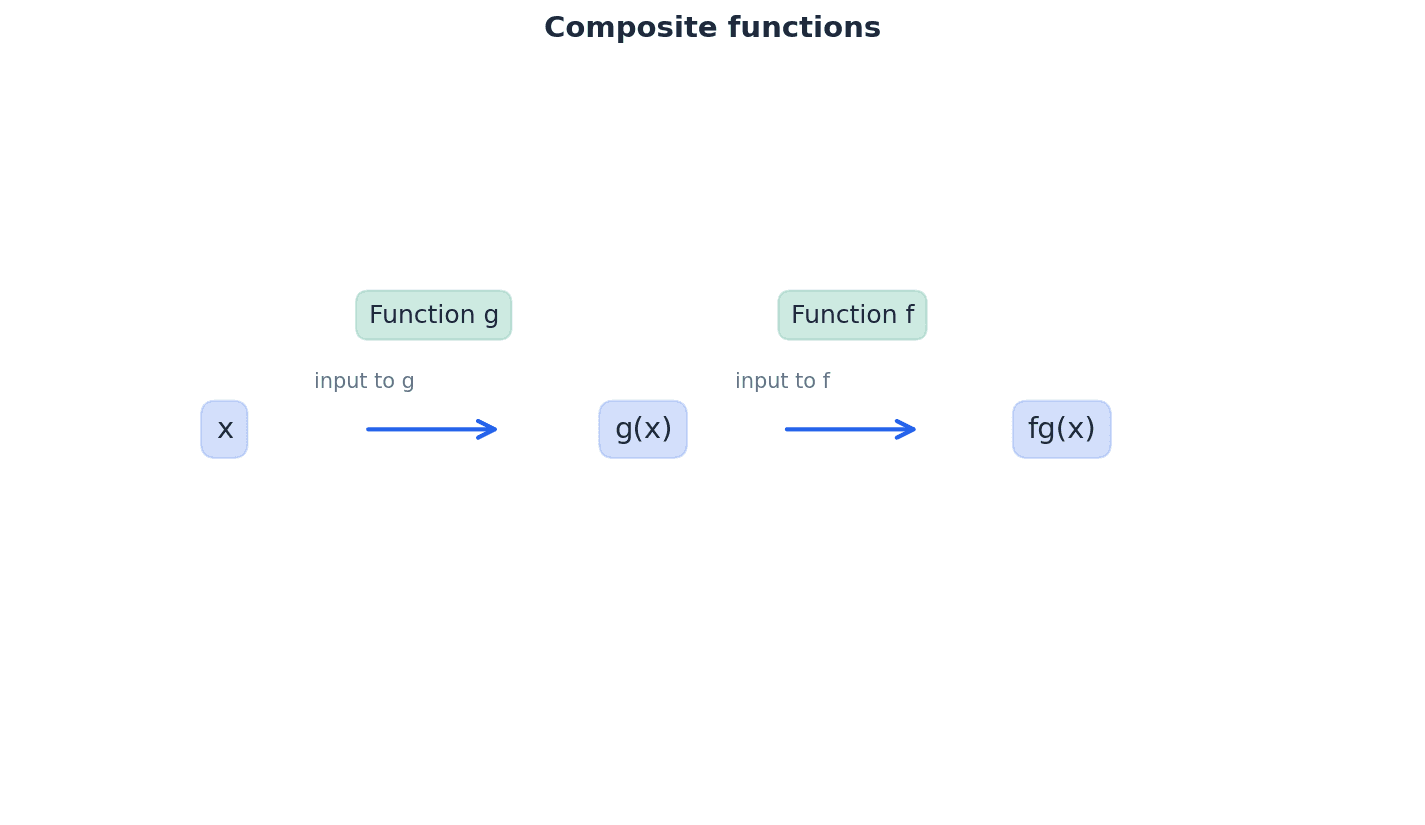
composite function — When one function is followed by another function, the resulting function is called a composite function.
A composite function, such as fg(x), means that function g acts on x first, and then function f acts on the result of g(x). The order of operations is crucial. Imagine a two-step process: first, you put clothes in a washing machine (function g), then you put them in a dryer (function f).
Remember that fg(x) only exists if the range of g is contained within the domain of f. Always check this condition, especially when dealing with restricted domains.
Students often confuse fg(x) with f(x) multiplied by g(x). It actually means f(g(x)), where the output of g becomes the input of f.
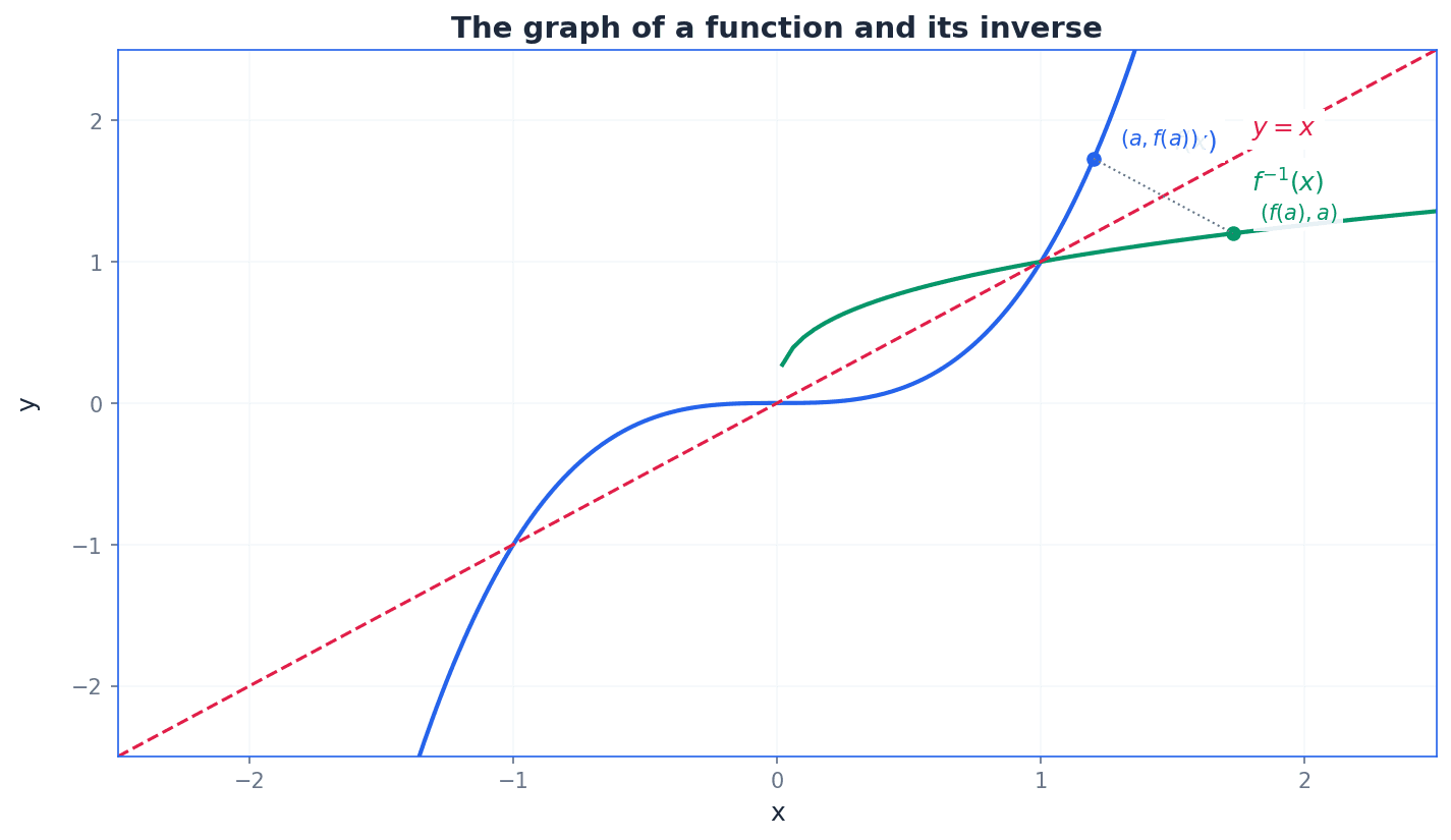
inverse function — The inverse of a function f(x) is the function that undoes what f(x) has done.
Written as f^-1(x), an inverse function reverses the mapping of the original function. If f maps x to y, then f^-1 maps y back to x. An inverse function only exists if the original function is one-one. If putting on your shoes is a function, then taking them off is its inverse function.
The domain of f^-1(x) is the range of f(x), and the range of f^-1(x) is the domain of f(x). This is a common point tested in exams.
Students often think f^-1(x) means 1/f(x). It actually denotes the inverse function, not the reciprocal.
self-inverse function — If f and f^-1 are the same function, then f is called a self-inverse function.
For a self-inverse function, applying the function twice returns the original input, i.e., ff(x) = x. Graphically, the graph of a self-inverse function is symmetrical about the line y = x. Flipping a coin is a self-inverse operation if you consider 'flipping' as the function.
transformation — Transformations are operations that change the position, size, or orientation of a graph.
This chapter covers translations, reflections, and stretches. Understanding these allows for predicting how a graph will change based on modifications to its function. Think of editing a photo: you can move it (translate), flip it (reflect), or resize it (stretch).
translation — A translation shifts the graph of a function without changing its shape or orientation.
The graph of y = f(x) + a is a vertical translation by (0, a), and y = f(x + b) is a horizontal translation by (-b, 0). This is like moving a picture frame on a wall without rotating or resizing it.
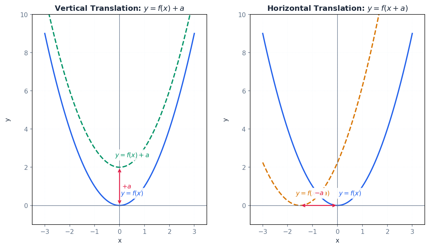
Students often confuse f(x+a) with f(x-a) for horizontal translations. Remember that f(x+a) shifts the graph 'a' units to the LEFT (negative x-direction), while f(x-a) shifts it 'a' units to the RIGHT (positive x-direction).
reflection — A reflection flips the graph of a function across an axis.
The graph of y = -f(x) is a reflection of y = f(x) in the x-axis. The graph of y = f(-x) is a reflection of y = f(x) in the y-axis. This is analogous to looking in a mirror.
Students sometimes mix up reflections in the x-axis and y-axis. Reflection in the x-axis affects the y-values (y becomes -y), while reflection in the y-axis affects the x-values (x becomes -x).
stretch — A stretch transforms the graph of a function by scaling it either vertically or horizontally.
The graph of y = af(x) is a stretch of y = f(x) with stretch factor 'a' parallel to the y-axis. The graph of y = f(ax) is a stretch of y = f(x) with stretch factor 1/a parallel to the x-axis. Imagine stretching a rubber band.
Students often confuse the stretch factor for horizontal stretches. For y = f(ax), the stretch factor is 1/a, not 'a'. This is because the x-values are effectively divided by 'a'.
When multiple transformations are applied to a function, the order of operations is crucial. Vertical transformations (affecting y-values) generally follow the normal order of operations, while horizontal transformations (affecting x-values) follow the opposite order. It is often helpful to break down combined transformations into individual steps and apply them sequentially to avoid errors.
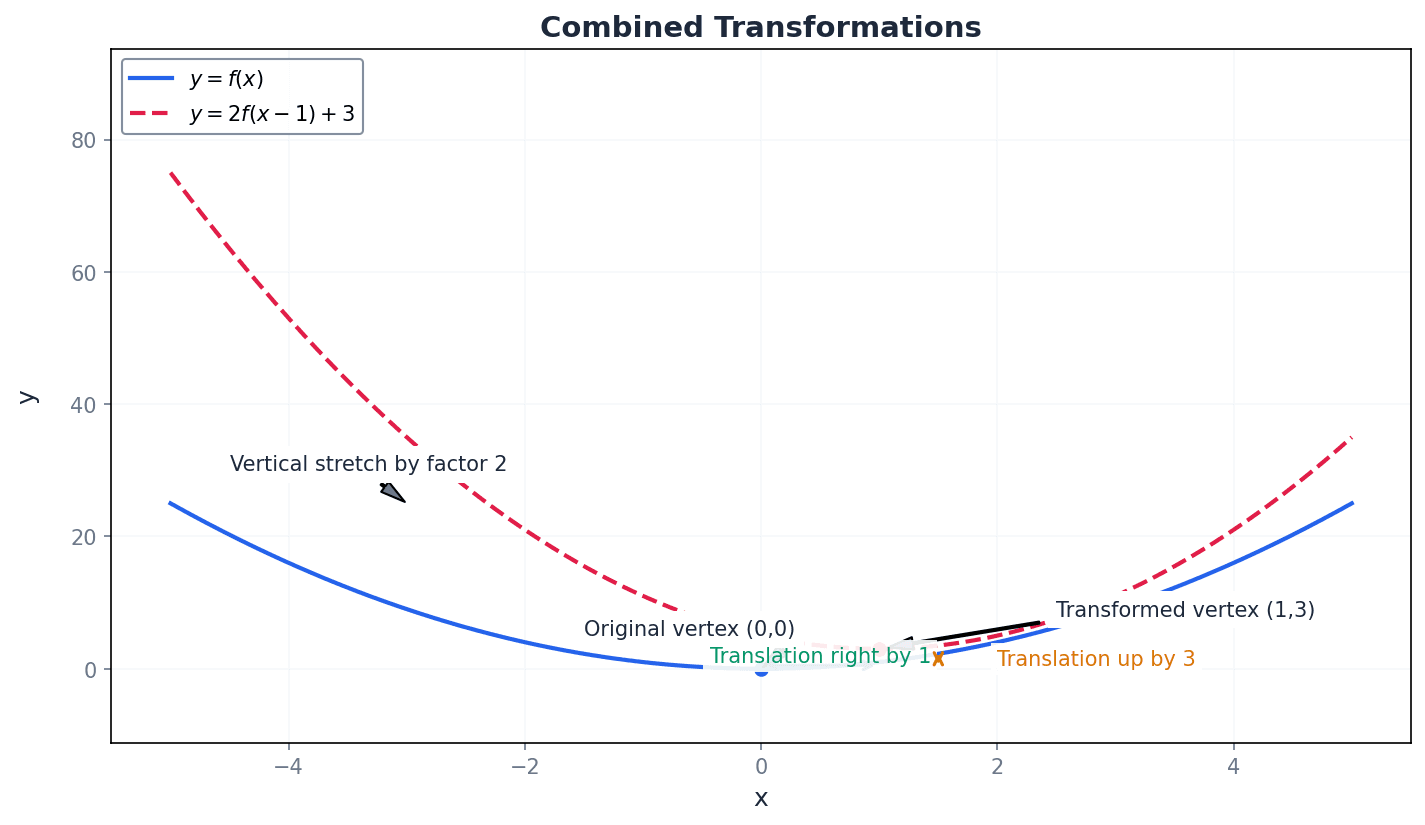
Students often apply transformations in the wrong order, especially when combining vertical and horizontal transformations or two transformations of the same type.
Always consider the order of transformations carefully. For combined transformations, it's often helpful to break them down into individual steps and apply them sequentially.
Clearly state the domain and range when defining a function or its inverse, as this is a common point tested in exams.
Exam Technique
Finding the range of a function
Finding a composite function fg(x)
| Mistake | Fix |
|---|---|
| Confusing fg(x) with f(x) multiplied by g(x). | Remember that fg(x) means f(g(x)), where the output of g becomes the input of f. Always substitute the entire function g(x) into f(x). |
| Assuming f^-1(x) means 1/f(x). | f^-1(x) denotes the inverse function, which 'undoes' f(x). It is not the reciprocal. To find it, swap x and y and rearrange. |
| Failing to check domain/range compatibility for composite functions. | For fg(x) to exist, the range of the inner function g must be contained within the domain of the outer function f. Always verify this condition. |
This chapter extends coordinate geometry concepts, covering calculations for length, midpoint, and gradient of line segments, and the equations of straight lines. It introduces the Cartesian equation of a circle and methods to find its centre and radius, culminating in solving problems involving the intersection of lines and circles.
conic section — A conic section is a curve obtained from the intersection of a plane with a cone.
Imagine shining a flashlight (a cone of light) onto a wall (a plane); the shape of the light on the wall is a conic section. There are three main types: ellipse, parabola, and hyperbola, with the circle being a special case of the ellipse. These curves are fundamental in astronomy and have reflective properties used in various optical designs.
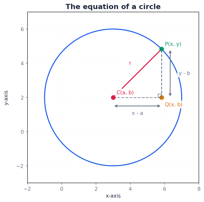
circle — A circle is defined as the locus of all the points in a plane that are a fixed distance (the radius) from a given point (the centre).
Imagine a dog tied to a post with a leash; the path the dog can walk, keeping the leash taut, forms a circle around the post. Its Cartesian equation is (x-a)^2 + (y-b)^2 = r^2, where (a, b) is the centre and r is the radius. It is a special case of an ellipse.
ellipse — The ellipse is one of the three types of conic section.
Imagine drawing a shape by tying a string to two pins and tracing with a pencil, keeping the string taut; that shape is an ellipse. It is a closed, oval shape, and the circle is considered a special case where the two foci coincide. Ellipses are important in describing planetary orbits.
parabola — The parabola is one of the three types of conic section.
The path of a ball thrown into the air (ignoring air resistance) follows a parabolic trajectory. It is a U-shaped curve, often seen as the graph of a quadratic function, and has unique reflective properties used in satellite dishes and searchlights.
hyperbola — The hyperbola is one of the three types of conic section.
Imagine the shadow cast by a lampshade on a wall; if the wall cuts through both the top and bottom cones of light, you'd see two separate hyperbolic curves. It consists of two disconnected curves, opening in opposite directions, and is used in navigation systems and some telescope designs.
P(x1, y1) — P(x1, y1) represents a point in the Cartesian coordinate system with x-coordinate x1 and y-coordinate y1.
Think of (x1, y1) as the 'address' of a specific house on a map. This notation distinguishes between different points, allowing for calculations of distance, gradient, and midpoint between them. The subscripts denote specific points.
Q(x2, y2) — Q(x2, y2) represents a second point in the Cartesian coordinate system with x-coordinate x2 and y-coordinate y2.
If P(x1, y1) is your starting point, then Q(x2, y2) is your destination point, and you can calculate the journey's length or halfway point. This notation is used with P(x1, y1) to define a line segment, enabling calculations of its length, midpoint, and gradient.
C(a, b) — C(a, b) represents the centre of a circle in the Cartesian coordinate system, with x-coordinate a and y-coordinate b.
If a circle is a Ferris wheel, C(a, b) is the central axle around which all the cabins rotate. The centre is the fixed point from which all points on the circumference are equidistant, and its coordinates are crucial for defining the circle's equation.
P(x, y) — P(x, y) represents a general point on the circumference of a circle or on a straight line.
If the circle is a path, P(x, y) is any specific spot you could be standing on that path. This notation is used to derive the general equation of a geometric shape, as 'x' and 'y' are variables that can take any value satisfying the equation for points on the shape.
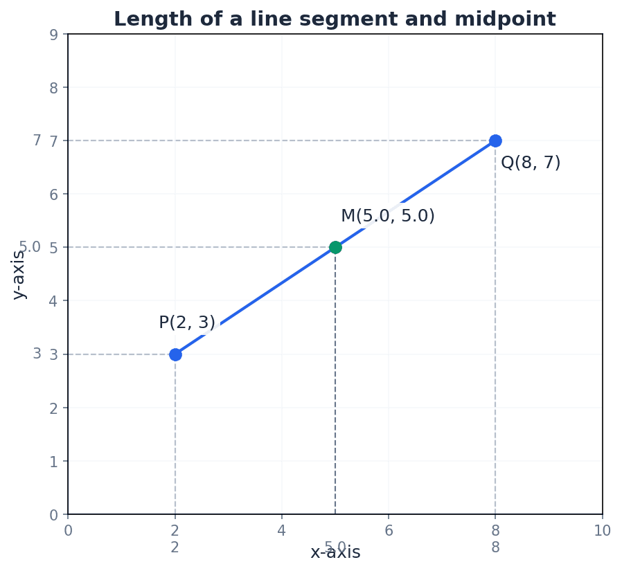
Coordinate geometry begins with understanding how to quantify properties of line segments. The length of a line segment between two points P(x1, y1) and Q(x2, y2) can be found using the distance formula, which is derived from Pythagoras' theorem. The midpoint, M, represents the point exactly halfway between P and Q, found by averaging their respective coordinates.
Length of a line segment
Used to calculate the distance between two given points P(x1, y1) and Q(x2, y2).
Midpoint of a line segment
Used to find the coordinates of the point exactly halfway between two given points P(x1, y1) and Q(x2, y2).
Clearly label your points (x1, y1) and (x2, y2) before applying formulae to avoid errors, especially in gradient calculations where the order matters for the sign.
Students often confuse x1 and x2, or y1 and y2, when applying formulas. Remember that while the order of points P and Q does not affect the final distance or midpoint, it does affect the sign of the gradient.
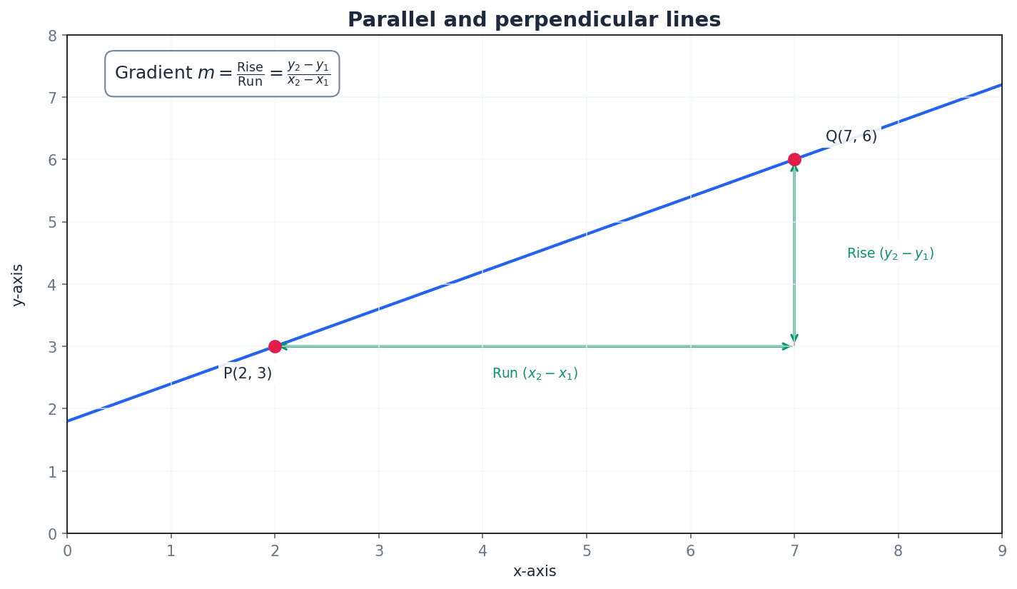
The gradient of a line, denoted by 'm', measures its steepness. It is calculated as the change in y-coordinates divided by the change in x-coordinates between two points on the line. This concept is crucial for determining relationships between lines, such as parallelism and perpendicularity.
Gradient of a line
Used to find the steepness of a line passing through two points P(x1, y1) and Q(x2, y2). For parallel lines, m1 = m2. For perpendicular lines, m1 * m2 = -1.
Two lines are parallel if they have the same gradient (m1 = m2). This means they maintain a constant distance from each other and never intersect. Conversely, two lines are perpendicular if the product of their gradients is -1 (m1 * m2 = -1), indicating they intersect at a right angle.
When finding the equation of a perpendicular bisector, students sometimes use the original line's gradient instead of the perpendicular gradient, or they use an endpoint instead of the midpoint. Always ensure you use the correct gradient and the midpoint for a perpendicular bisector.
When calculating gradients or lengths, ensure you consistently subtract the coordinates in the same order (e.g., x2 - x1 and y2 - y1) to avoid errors.
The equation of a straight line can be expressed in various forms. The gradient-intercept form, y = mx + c, is useful when the gradient 'm' and y-intercept 'c' are known. Alternatively, the point-gradient form, y - y1 = m(x - x1), is effective when a point (x1, y1) and the gradient 'm' are given. Vertical lines have a special form, x = b, where 'b' is the x-intercept.
Equation of a straight line (gradient-intercept form)
Used when the line is non-vertical. 'c' is the point where the line crosses the y-axis.
Equation of a vertical straight line
Used when the line is vertical. 'b' is the point where the line crosses the x-axis.
Equation of a straight line (point-gradient form)
Used to find the equation of a line when its gradient 'm' and a point (x1, y1) on the line are known.
A circle is defined by its centre C(a, b) and its radius r. Its Cartesian equation in completed square form is (x-a)^2 + (y-b)^2 = r^2, directly derived from Pythagoras' theorem. This form clearly shows the centre and radius. The equation can also be expanded into a general form, x^2 + y^2 + 2gx + 2fy + c = 0, from which the centre (-g, -f) and radius sqrt(g^2 + f^2 - c) can be found by completing the square.
Equation of a circle (completed square form)
Represents a circle with centre (a, b) and radius r. This form is derived directly from Pythagoras' theorem.
Equation of a circle (expanded general form)
Represents a circle with centre (-g, -f) and radius sqrt(g^2 + f^2 - c). This form is obtained by expanding the completed square form.
Students often forget that in the equation (x-a)^2 + (y-b)^2 = r^2, the signs of 'a' and 'b' are reversed when identifying the centre, e.g., (x+2)^2 means a = -2. Always be careful with the signs when extracting the centre coordinates.
When asked to find the equation of a circle, ensure you identify both the centre coordinates and the radius, as both are required for full marks.
Problems involving the intersection of lines and circles are solved using simultaneous equations. By substituting the linear equation into the circle's equation, a quadratic equation is formed. The discriminant (b^2 - 4ac) of this quadratic determines the nature of the intersection: a positive discriminant indicates two distinct points, a zero discriminant indicates a tangent (one repeated root), and a negative discriminant means no intersection.
Students may incorrectly assume that if a line intersects a curve, it will always result in two distinct points, forgetting the case of a tangent (one repeated root) or no intersection (no real roots). Always consider the discriminant.
When completing the square for a circle's equation, students might forget to subtract the added constant terms, leading to an incorrect radius squared value. Remember to balance the equation.
Always show all steps of your algebraic working clearly, especially for calculations of length, midpoint, and gradient. Do not rely on scale drawings.
For intersection problems, set up simultaneous equations and use the discriminant to determine the number of intersection points if required.
Practice finding equations of perpendicular bisectors, as this combines multiple concepts: midpoint, perpendicular gradient, and line equation.
Exam Technique
Find the midpoint of a line segment
Find the length of a line segment
| Mistake | Fix |
|---|---|
| Forgetting to show appropriate calculations and relying on scale drawings. | Always perform and present full algebraic working for all coordinate geometry questions. Scale drawings are not sufficient for marks. |
| Sign errors when extracting centre coordinates (a, b) from (x-a)^2 + (y-b)^2 = r^2. | Remember that the signs are reversed. For (x+a)^2, the x-coordinate of the centre is -a. Double-check signs carefully. |
| Using the original line's gradient or an endpoint instead of the perpendicular gradient and midpoint for a perpendicular bisector. | Always calculate the perpendicular gradient (m1 * m2 = -1) and the midpoint of the line segment. The perpendicular bisector passes through the midpoint with the perpendicular gradient. |
This chapter introduces radians as an alternative unit for measuring angles, alongside degrees, and explains the conversion between them. It then develops and applies formulae for calculating the arc length and area of a sector of a circle, emphasizing that these formulae require angles to be in radians. The chapter also covers related geometric concepts such as chords, segments, and the distinction between minor and major parts of a circle.
centre — The centre of a circle is the point equidistant from all points on its circumference.
This is the central point from which all radii extend. Angles subtended by arcs and sectors are measured from the centre, making its location crucial for calculations.
radius — The radius of a circle is the distance from its centre to any point on its circumference.
The radius is a fundamental property of a circle, akin to a spoke on a bicycle wheel. It is used in calculating circumference, area, arc length, and sector area, and all radii in a given circle have the same length.
radian — One radian is the size of the angle subtended at the centre of a circle, radius r, by an arc of length r.
Radians are an alternative unit for measuring angles, often referred to as the natural unit of angular measure. Imagine a piece of string exactly the length of a circle's radius; if you lay that string along the circumference, the angle it 'cuts out' from the center is 1 radian. They simplify many mathematical formulae and calculations, especially in calculus, with one complete revolution being 2π radians.
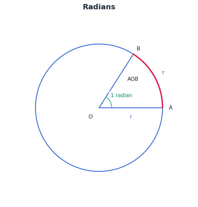
Angles can be measured in degrees or radians. Radians are based on the geometric relationship between the arc length and radius, making them fundamental in higher mathematics. One complete revolution is 2π radians, which is equivalent to 360 degrees.
Degrees to Radians Conversion
Used to convert an angle from degrees to radians.
Radians to Degrees Conversion
Used to convert an angle from radians to degrees.
Students often confuse degrees and radians, leading to incorrect calculations if the calculator mode is not set correctly. Always check your calculator's mode (degrees or radians) before solving problems involving trigonometric functions or circular measure.
Always check your calculator's mode (degrees or radians) before solving problems involving trigonometric functions or circular measure, as using the wrong mode is a common error.
arc length — The length of an arc is the distance along the curved edge of a sector or segment of a circle.
For an angle θ measured in radians, the arc length is directly proportional to both the radius and the angle. This formula is derived from the definition of a radian, where an arc equal to the radius subtends 1 radian. If you cut a slice of pizza, the arc length is the length of the crust on that slice.
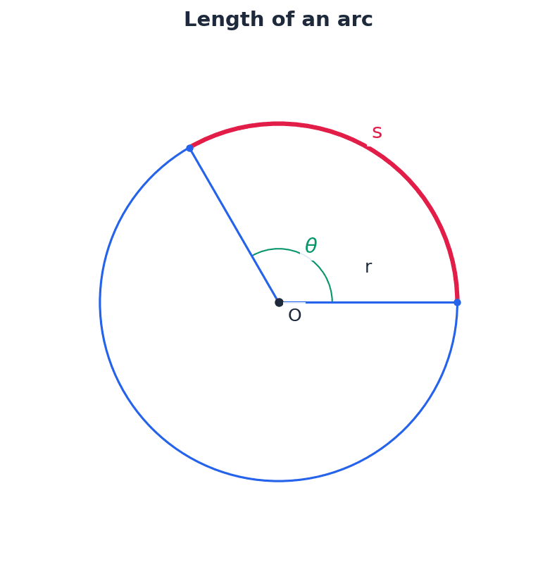
Arc Length
Used to calculate the length of an arc when the angle is measured in radians. This formula is only valid when θ is measured in radians.
Students often use the arc length formula with angles in degrees, but the formula s = rθ is only valid when θ is in radians. If given in degrees, convert it first using the conversion factor π/180.
When calculating arc length, ensure the angle is in radians. If given in degrees, convert it first using the conversion factor π/180.
sector — A sector of a circle is the region bounded by two radii and the arc connecting their endpoints.
It resembles a 'slice' of a circle, like a slice of a round cake or pizza. The area of a sector is a fraction of the total area of the circle, determined by the ratio of the sector's angle to the complete angle at the centre.
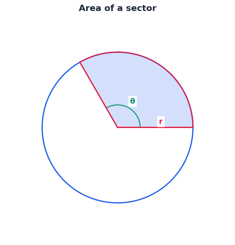
Area of Sector
Used to calculate the area of a sector when the angle is measured in radians. This formula is only valid when θ is measured in radians.
Students often use the sector area formula with angles in degrees, but the formula A = 1/2 r²θ is only valid when θ is in radians.
chord — A chord is a straight line segment connecting two points on the circumference of a circle.
A chord is like a straight bridge connecting two points on the edge of a circular pond. It divides the circle into two segments. The longest chord in a circle is its diameter.
minor arc — A minor arc is the shorter of the two arcs connecting two points on a circle's circumference.
When a chord divides a circle, it creates two arcs. The minor arc is the one that subtends an angle less than π radians (180 degrees) at the centre. If you draw a line across a circle, the minor arc is the smaller curve between the two points where the line touches the circle.
major arc — A major arc is the longer of the two arcs connecting two points on a circle's circumference.
It subtends a reflex angle (greater than π radians or 180 degrees) at the centre. The length of the major arc is the circumference minus the length of the minor arc. Using the pizza slice analogy, if the minor arc is the crust of a small slice, the major arc is the rest of the crust of the pizza.
minor sector — A minor sector is the smaller region of a circle bounded by two radii and the minor arc.
It corresponds to an angle less than π radians (180 degrees) at the centre. Its area is calculated using the formula for sector area with the minor angle. A minor sector is a standard, smaller slice of a pie.
major sector — A major sector is the larger region of a circle bounded by two radii and the major arc.
It corresponds to a reflex angle (greater than π radians or 180 degrees) at the centre. Its area can be found by subtracting the minor sector area from the total circle area, or by using the reflex angle in the sector area formula. A major sector is the larger part of a pie after a small slice has been removed.
Students often misinterpret 'minor' and 'major' arcs/sectors/segments, using the wrong angle (θ vs. 2π - θ) in calculations. Remember that for major arcs or sectors, the angle will be 2π - θ (or 360° - θ if working in degrees for other parts of the problem).
Be careful to distinguish between minor and major sectors; the question will usually specify or imply which one is required. The angle for a major sector will be (2π - θ) if θ is the minor angle.
minor segment — A minor segment is the smaller region of a circle bounded by a chord and its corresponding minor arc.
Its area is found by subtracting the area of the triangle formed by the chord and the two radii from the area of the minor sector. A minor segment is the part of a pizza slice that remains after you cut off the triangular part (the part with the crust).
major segment — A major segment is the larger region of a circle bounded by a chord and its corresponding major arc.
Its area can be found by adding the area of the triangle formed by the chord and the two radii to the area of the major sector, or by subtracting the minor segment area from the total circle area. A major segment is the larger part of a pizza after a small segment has been removed.
Students often confuse the terms 'sector' and 'segment', and their respective area calculations. A sector is bounded by two radii and an arc, while a segment is bounded by a chord and an arc.
Students often forget to subtract the area of the triangle from the sector area when calculating the area of a segment. To find the area of a minor segment, calculate the area of the minor sector and then subtract the area of the isosceles triangle formed by the two radii and the chord.
To find the area of a minor segment, calculate the area of the minor sector and then subtract the area of the isosceles triangle formed by the two radii and the chord.
For segment area problems, clearly show the calculation for the sector area and the triangle area separately.
Always ensure you are using the correct value for the radius (r) in formulas, especially when the diameter is given, as this is a common source of error.
Double-check your calculator is in the correct mode (radians or degrees) before performing any calculations.
Exam Technique
Convert Degrees to Radians
Convert Radians to Degrees
| Mistake | Fix |
|---|---|
| Using degrees instead of radians in arc length and sector area formulas. | Always convert angles to radians before using s = r\theta and A = \frac{1}{2}r^2\theta. Double-check your calculator's mode. |
| Confusing sectors and segments. | Remember a sector includes the radii to the center, while a segment is bounded by a chord and an arc. Their area calculations are different. |
| Forgetting to subtract the triangle area when finding segment area. | The area of a segment is the area of the sector minus the area of the triangle formed by the radii and the chord. |
This chapter explores trigonometric functions for any angle, covering their graphs, exact values, and transformations. It introduces fundamental identities and inverse functions, providing methods for solving trigonometric equations within specified intervals.
Periodic functions — Functions that repeat themselves over and over again.
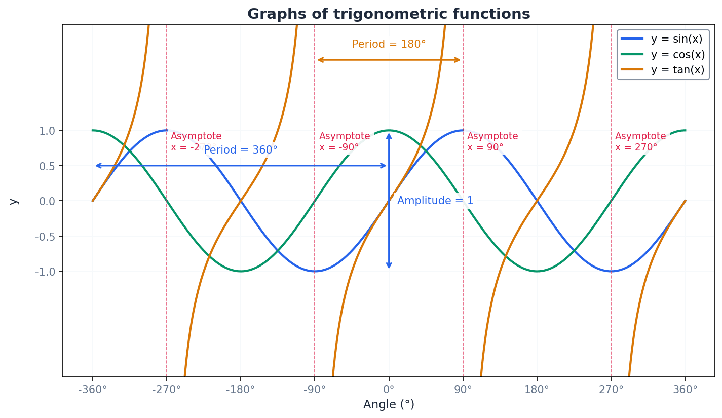
The sine and cosine functions are examples of periodic functions, repeating their pattern every 360° (or 2π radians). This property is crucial for modelling wave phenomena, much like the hands of a clock repeat their positions every 12 hours.
Period — The length of one repetition or cycle of a periodic function.
For sine and cosine functions, the period is 360° (or 2π radians), meaning the graph completes one full cycle and starts repeating after this interval. For the tangent function, the period is 180° (or π radians). This is like the distance you travel on a circular track to get back to your starting point.
Students often think the period is always 360° for all trigonometric functions, but actually the tangent function has a period of 180°.
Amplitude — The distance between a maximum (or minimum) point and the principal axis of a periodic function.
For y = sinx and y = cosx, the amplitude is 1. Transformations like y = Asinx change the amplitude to |A|. The tangent function does not have an amplitude. Imagine a swing; the amplitude is how far the swing goes from its resting position to its highest point.
Students often think the amplitude is the distance from the minimum to the maximum, but actually it's half that distance, from the principal axis to the max/min.
Asymptotes — Lines that the branches of a graph get closer and closer to without ever reaching them.
For the tangent function, vertical asymptotes occur at 90°, 270°, and so on, because tanx is undefined at these angles. These lines indicate where the function's value approaches infinity, like a car approaching a wall but never quite touching it.
When sketching tangent graphs, always draw and label the asymptotes as dashed lines to clearly show the function's behaviour.
Identity — An equation that is true for all values of the variable.
Trigonometric identities like tanθ ≡ sinθ/cosθ and sin²θ + cos²θ ≡ 1 are fundamental relationships that hold true for any valid angle θ. They are used to simplify expressions and prove other identities, much like saying 'a square is a rectangle with four equal sides' – it's always true by definition.
Students often confuse identities with equations, but actually identities are true for all values, while equations are true only for specific values.
Tangent Identity
True for all θ where cosθ ≠ 0.
Pythagorean Identity
True for all θ.
Angles can be of any size, measured in degrees or radians. For a point P(x,y) on a circle of radius r centered at the origin, the trigonometric ratios are generally defined. This allows us to extend the concept of trigonometry beyond acute angles in right-angled triangles.
General Sine Definition
For a point P(x,y) on a circle of radius r centered at the origin.
General Cosine Definition
For a point P(x,y) on a circle of radius r centered at the origin.
General Tangent Definition
For a point P(x,y) on a circle of radius r centered at the origin, where x ≠ 0.
Acute angle — An angle between 0° and 90°.
In trigonometry, the 'basic angle' or 'reference angle' is always an acute angle. This acute angle is like a building block, used to find trigonometric ratios for angles in other quadrants by considering symmetry.
Always identify the basic acute angle first when dealing with angles outside the first quadrant, as it simplifies finding the value of the trigonometric ratio.
The Cartesian plane is divided into four quadrants, and the signs of sine, cosine, and tangent vary depending on which quadrant the angle lies in. Understanding these signs is crucial for solving equations and expressing ratios of general angles in terms of acute angles.
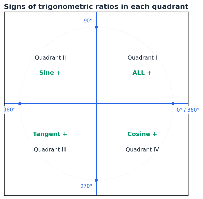
First quadrant — The region of the Cartesian plane where both x and y coordinates are positive.
In this quadrant, all three basic trigonometric ratios (sine, cosine, tangent) are positive. Angles in this quadrant are between 0° and 90° (or 0 and π/2 radians). It's like the 'all clear' zone on a map, where everything is positive and straightforward.
Second quadrant — The region of the Cartesian plane where x coordinates are negative and y coordinates are positive.
In this quadrant, only the sine ratio is positive, while cosine and tangent are negative. Angles in this quadrant are between 90° and 180° (or π/2 and π radians). Think of it as the 'sine-only' zone, where sine gets special positive treatment.
Third quadrant — The region of the Cartesian plane where both x and y coordinates are negative.
In this quadrant, only the tangent ratio is positive, while sine and cosine are negative. Angles in this quadrant are between 180° and 270° (or π and 3π/2 radians). This is the 'tangent's turn' zone, where it's the only one with a positive value.
Fourth quadrant — The region of the Cartesian plane where x coordinates are positive and y coordinates are negative.
In this quadrant, only the cosine ratio is positive, while sine and tangent are negative. Angles in this quadrant are between 270° and 360° (or 3π/2 and 2π radians). This is the 'cosine's domain', where it reigns supreme with a positive value.
Students may make sign errors for trigonometric ratios in different quadrants. Use the 'All Students Trust Cambridge' mnemonic to quickly recall which ratios are positive in each quadrant.
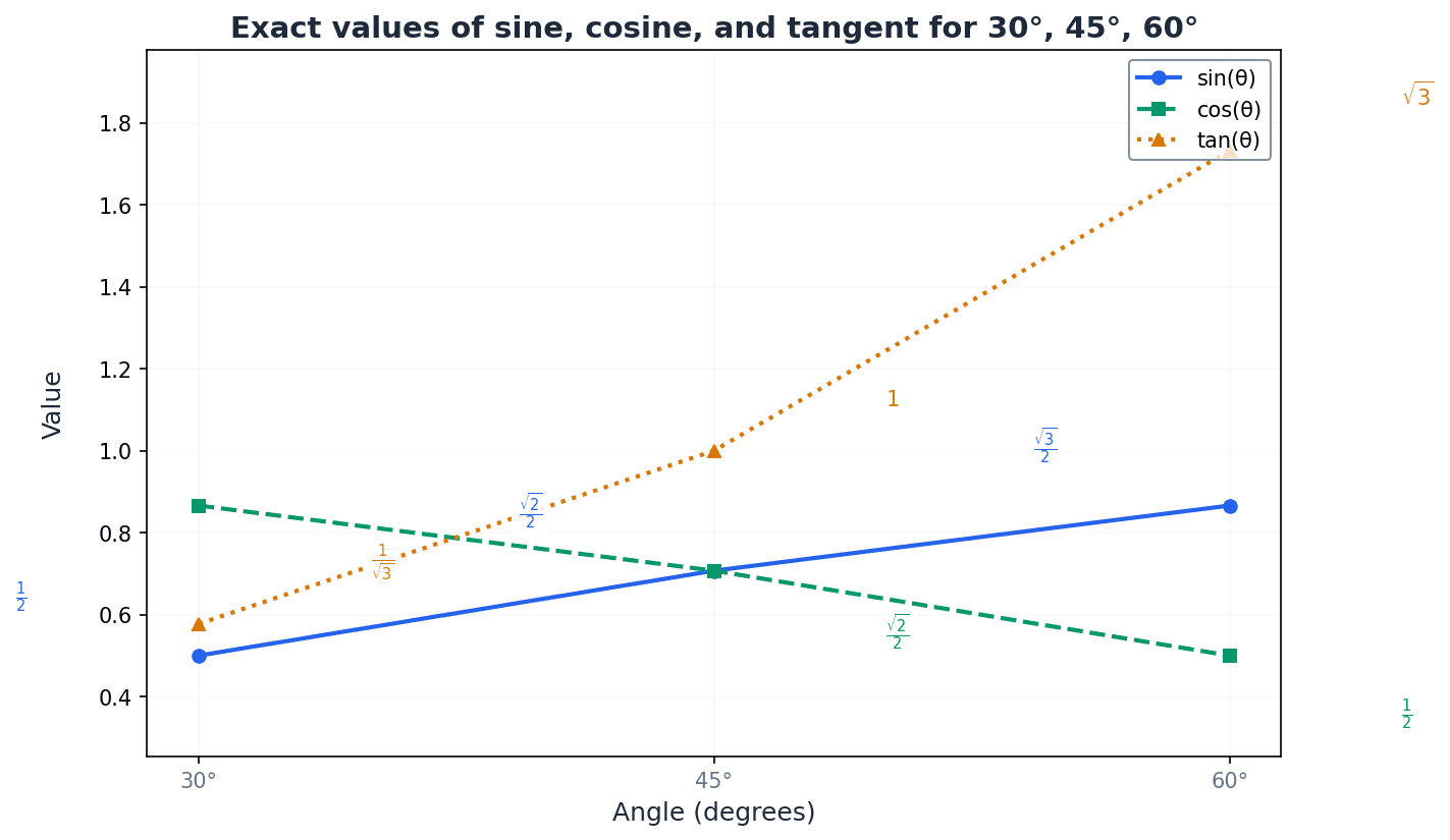
It is essential to know the exact values of sine, cosine, and tangent for specific acute angles such as 30°, 45°, and 60°. These values, along with the understanding of quadrant signs, allow for the calculation of exact trigonometric ratios for related angles in all four quadrants without a calculator.
The graphs of sine, cosine, and tangent functions visually represent their periodic nature and values for angles of any size. Sketching these graphs is fundamental for understanding their properties, such as period, amplitude, and asymptotes, and for visualising solutions to trigonometric equations.
When sketching periodic functions, ensure you show at least one full cycle and correctly label the period and amplitude.
Trigonometric graphs can be transformed through translations, stretches, and reflections, similar to other functions. Understanding these transformations allows for sketching more complex trigonometric functions based on the basic sine, cosine, and tangent curves. For example, y = sin(x-90°) is a horizontal translation of y = sinx by 90° to the right.
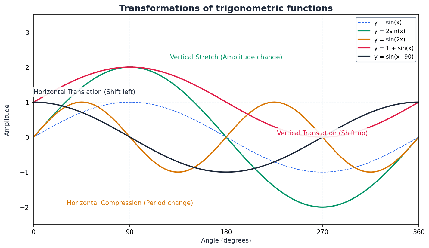
When asked to find the period of a transformed function like sin(ax), remember the period is 360°/a (or 2π/a), not 360°.
Inverse function — A function that 'reverses' the action of another function.
For trigonometric functions, inverse functions (sin⁻¹, cos⁻¹, tan⁻¹) are defined by restricting the domain of the original function to make it one-to-one, ensuring a unique output for each input. This is like taking off your socks after putting them on.
Students often think sin⁻¹x is the same as 1/sinx, but actually sin⁻¹x denotes the inverse function, not the reciprocal.
Principal angle — The angle that lies in the range of the inverse trigonometric function.
When solving trigonometric equations using inverse functions (e.g., sin⁻¹x), a calculator typically provides only one solution, which is the principal angle. Other solutions must be found using the function's periodicity and symmetry. This is like asking for 'the' capital of a country, you get one specific answer.
Students frequently forget to consider all quadrants when solving trigonometric equations, only providing the principal value from the calculator.
Solving trigonometric equations involves finding all angles that satisfy a given equation within a specified interval. This often requires using fundamental identities, understanding the signs of ratios in different quadrants, and applying the periodicity of the functions to find all possible solutions.
Always sketch the graph of the relevant trigonometric function to visualise all possible solutions within the given interval.
When proving an identity, start with the more complicated side and manipulate it algebraically until it matches the simpler side; do not treat it as an equation by operating on both sides simultaneously.
Pay close attention to the specified interval for solutions; ensure all solutions found lie within this range.
Exam Technique
Finding exact values of trigonometric ratios for general angles
Proving trigonometric identities
| Mistake | Fix |
|---|---|
| Confusing sin⁻¹x with 1/sinx. | Remember that sin⁻¹x denotes the inverse function, which gives an angle, while 1/sinx is the reciprocal, cosecx. |
| Only providing the principal value from a calculator when solving trigonometric equations. | Always consider all quadrants and the periodicity of the function to find all possible solutions within the specified interval. Sketching the graph helps visualise this. |
| Assuming the period of tanx is 360°. | The period of tanx is 180° (or π radians). This is a key difference from sinx and cosx. |
This chapter introduces the concept of series, focusing on binomial expansions, arithmetic progressions, and geometric progressions. It covers methods for expanding binomial expressions, provides formulae for finding the nth term and sum of the first n terms for both arithmetic and geometric progressions, and explores infinite geometric series, including their convergence condition and sum to infinity.
Series — When the terms in a sequence are added together we call the resulting sum a series.
A series is the sum of the terms of a sequence. For arithmetic and geometric progressions, specific formulae exist to calculate the sum of the first 'n' terms. A sequence is like a list of ingredients, while a series is like the total weight or cost of all those ingredients combined.
Students often confuse 'sequence' and 'series'. Remember that a sequence is a list of numbers, while a series is the sum of those numbers.
Binomial — Binomial means 'two terms'.
In algebra, expressions with two terms, such as (a+b), are called binomials. The binomial expansion refers to the process of expanding such expressions raised to a positive integer power. Think of 'bi' as in 'bicycle' (two wheels); a binomial has two parts or terms.
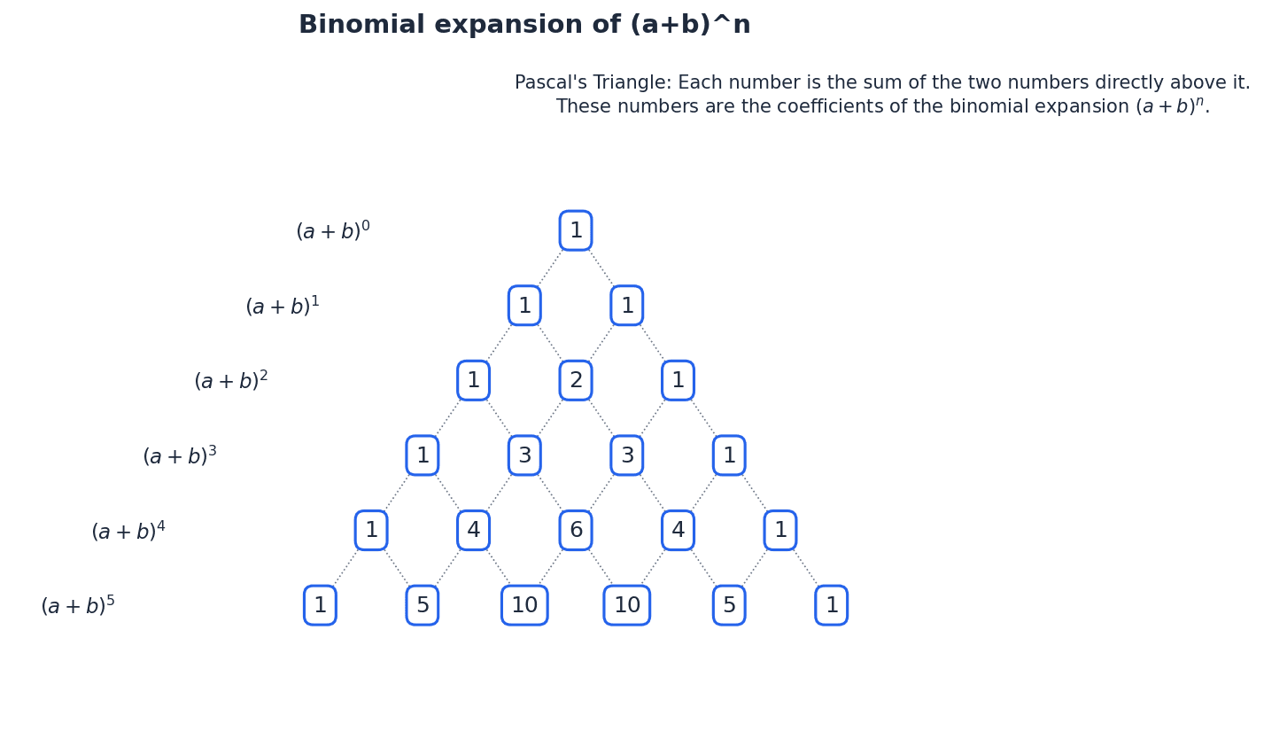
Binomial coefficients — The coefficients in the binomial expansion of (a+x)^n are known as binomial coefficients.
These coefficients determine the numerical part of each term in a binomial expansion. They can be found using Pascal's triangle or the nCr formula, and are crucial for calculating specific terms without full expansion. Binomial coefficients are like the 'recipe' for how many times each combination of 'a' and 'x' appears when you multiply out a binomial expression.
Pascal’s triangle — The coefficients also form a pattern that is known as Pascal’s triangle.
Pascal's triangle is a triangular array of binomial coefficients, where each number is the sum of the two numbers directly above it. It provides a quick way to find coefficients for binomial expansions with small positive integer powers. Imagine a pyramid of numbers where each brick is the sum of the two bricks above it; that's how Pascal's triangle builds its rows of coefficients.
Factorial notation
Represents the product of all positive integers up to n. 0! is defined as 1.
Binomial Coefficient (nCr) formula
Used to calculate binomial coefficients without Pascal's triangle, where n is a positive integer and r is a positive integer less than n.
The binomial expansion allows us to expand expressions of the form (a+b)^n, where 'n' is a positive integer. The coefficients for each term in this expansion are known as binomial coefficients, which can be determined using Pascal's triangle or the nCr formula. The powers of 'a' decrease while the powers of 'b' increase, ensuring the total index remains 'n' for each term.
Binomial Theorem (positive integer n)
Used for expanding binomials raised to a positive integer power. The (r+1)th term is \binom{n}{r}a^{n-r}b^r.
Binomial Theorem (simplified for (1+x)^n)
A special case of the Binomial Theorem when the first term is 1. The (r+1)th term is \binom{n}{r}x^r.
When asked to expand a binomial, ensure all terms are included and powers of 'a' decrease while powers of 'b' increase, maintaining the correct total index.
When expanding (a-b)^n, students often forget to correctly handle the negative sign for the 'b' term, especially with even powers. Be careful with negative signs and powers.
Students might assume that binomial coefficients are only for (1+x)^n. Remember that they apply to (a+x)^n as well, though the 'a' term needs to be factored in.
Arithmetic progression — A linear sequence such as 5, 8, 11, 14, 17, … is also called an arithmetic progression.
In an arithmetic progression, each term differs from the preceding term by a constant value, known as the common difference. This type of sequence models linear growth or decay. Think of climbing a ladder where each rung is the same distance apart; the height of each rung forms an arithmetic progression.
Common difference — Each term differs from the term before by a constant. This constant is called the common difference.
The common difference (d) is the constant value added to each term to get the next term in an an arithmetic progression. It can be positive, negative, or zero. It's like the fixed step size you take when walking; each step adds the same distance to your total journey.
Students often think the common difference must be positive. Remember that it can be zero or negative, leading to constant or decreasing sequences.
nth term of an arithmetic progression
Used to find any term in an arithmetic progression, where 'a' is the first term and 'd' is the common difference.
Sum of the first n terms of an arithmetic progression (Sn)
Used when the first term 'a' and last term 'l' are known.
Sum of the first n terms of an arithmetic progression (Sn, alternative)
Used when the first term 'a' and common difference 'd' are known.
When solving problems involving arithmetic progressions, clearly identify the first term (a) and common difference (d) before applying the nth term or sum formulae.
Geometric progression — The sequence 2, 6, 18, 54, … is called a geometric progression.
In a geometric progression, each term is found by multiplying the preceding term by a constant value, known as the common ratio. This type of sequence models exponential growth or decay. Imagine a chain reaction where each step multiplies the previous outcome; the results form a geometric progression.
Common ratio — Each term is three times the preceding term. The constant multiplier, 3, is called the common ratio.
The common ratio (r) is the constant value by which each term is multiplied to get the next term in a geometric progression. It can be positive or negative, an integer or a fraction. It's like the scaling factor in a photocopy machine; each copy is a certain multiple of the original size.
Students often think the common ratio must be an integer. Remember that it can be a fraction, a decimal, or even negative.
nth term of a geometric progression
Used to find any term in a geometric progression, where 'a' is the first term and 'r' is the common ratio.
Sum of the first n terms of a geometric progression (Sn, r > 1)
Used when the common ratio r is greater than 1.
Sum of the first n terms of a geometric progression (Sn, r < 1)
Used when the common ratio r is less than 1 (or when |r| < 1).
When dealing with geometric progressions, ensure you correctly identify the common ratio (r) by dividing a term by its preceding term (e.g., term2 / term1).
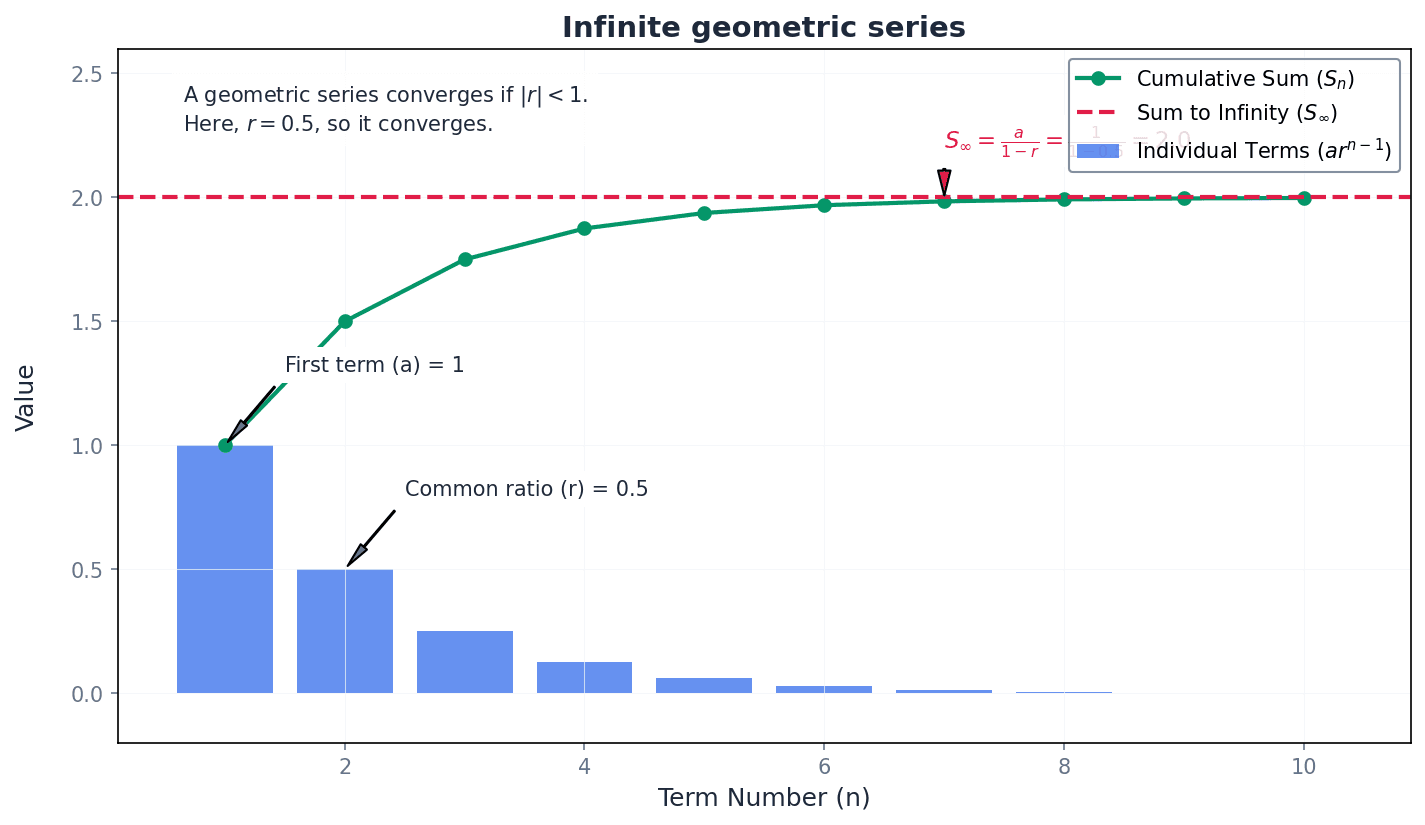
Convergent series — A series that converges is also known as a convergent series.
An infinite geometric series is convergent if the sum of its terms approaches a finite limit as the number of terms tends to infinity. This occurs when the absolute value of the common ratio is less than 1. Imagine repeatedly cutting a piece of string in half and adding the lengths; the total length will approach the original length of the string, but never exceed it.
Sum to infinity of a geometric progression (S_infinity)
Used only when the geometric series converges, i.e., when |r| < 1.
Students may incorrectly apply the sum to infinity formula for a geometric series when the condition |r| < 1 is not met. Always check this condition first.
Always check the condition |r| < 1 before attempting to calculate the sum to infinity of a geometric series; if this condition is not met, the series does not converge.
Relationship between Sn and un
Applies for all sequences to find the nth term from the sum of terms.
Distinguish carefully between finding the nth term of a sequence and finding the sum of a series; different formulae apply.
When finding the common difference or common ratio, students sometimes subtract/divide in the wrong order, leading to incorrect signs or values. Always calculate by subtracting a term from its subsequent term (e.g., term2 - term1) or dividing a term by its preceding term (e.g., term2 / term1).
When solving problems involving both arithmetic and geometric progressions, students may mix up the respective formulae for nth term or sum. Clearly state whether a progression is arithmetic or geometric before applying formulae.
For problems involving both AP and GP, ensure you use the correct set of formulae for each part. Practice problems involving finding 'n' when given S_n or u_n, as this often requires solving quadratic equations.
Exam Technique
Expanding (a+b)^n using Pascal's Triangle
Finding a specific term or coefficient in a binomial expansion
| Mistake | Fix |
|---|---|
| Confusing 'sequence' and 'series'. | Remember a sequence is a list of numbers, while a series is the sum of those numbers. |
| Incorrectly handling negative signs in binomial expansions like (a-b)^n. | Treat 'b' as '-b' in the formula, ensuring that even powers of '-b' become positive and odd powers remain negative. |
| Applying the sum to infinity formula for a geometric series when it does not converge. | Always check the condition |r| < 1 before using S_\infty = a/(1-r). If |r| >= 1, the series does not have a finite sum to infinity. |
Differentiation is a fundamental calculus tool for finding the exact gradient of a curve at any point, building on the concept of limits of chord gradients. This chapter covers essential differentiation rules and their application to finding equations of tangents and normals, as well as calculating second derivatives.
differentiation — The process of finding the gradient of a curve at any point.
Differentiation is one of the two basic tools of calculus, used to study rates of change. It allows for finding the exact gradient of a curve, unlike approximate methods like drawing tangents. Imagine you're driving a car and want to know your exact speed at a particular instant. Differentiation is like having a perfect speedometer that tells you the instantaneous speed, rather than just your average speed over a period.
derivative — The result of differentiating a function, representing the gradient function of the curve.
The derivative, denoted as dy/dx or f'(x), gives a formula that can be used to calculate the gradient of the tangent to the curve at any given x-coordinate. It is a function itself. If a function describes the height of a roller coaster over time, its derivative describes the steepness of the roller coaster at any given moment.
gradient function — Another name for the derivative of a curve, as it provides the gradient at any point on the curve.
If y = f(x) is the graph of a function, then dy/dx or f'(x) is sometimes also called the gradient function of this curve. It allows for calculating the slope of the tangent at any point without drawing. Think of a map where each point has a number indicating its elevation. The gradient function is like another map that, for every point, tells you how steep the terrain is in a particular direction.
Students often think differentiation only applies to straight lines, but actually it is specifically for finding the gradient of curves at a single point.
Students often think the derivative is a single number, but actually it is a function that gives the gradient at any point, unless evaluated at a specific x-value.
Power Rule for Differentiation
Multiply by the power n and then subtract one from the power. This rule applies for any rational power n.
Scalar Multiple Rule
The derivative of a constant times a function is the constant times the derivative of the function.
Addition/Subtraction Rule
The derivative of a sum or difference of functions is the sum or difference of their derivatives.
The gradient of a curve at a point is understood as the limit of the gradients of a suitable sequence of chords. Differentiation provides a precise method for finding this exact gradient. The result of this process is the derivative, also known as the gradient function, which gives a formula for the gradient at any point on the curve.
When asked to 'differentiate from first principles', ensure you show the limit of the gradients of chords, as this demonstrates understanding of the fundamental definition, not just the rules.
Be precise with notation; dy/dx refers to the derivative of y with respect to x, while f'(x) refers to the derivative of the function f(x). Using the correct notation is crucial for clarity and marks.
Students often think the gradient function is the same as the original function, but actually it describes the rate of change of the original function, not its values.
The power rule, , is fundamental for differentiating functions of the form , including those with fractional or negative powers. When differentiating expressions involving sums or differences of functions, the addition/subtraction rule allows each term to be differentiated separately. For terms multiplied by a constant, the scalar multiple rule states that the constant can be factored out before differentiation.
Failing to simplify expressions (e.g., as , as ) before differentiating is a common error. Always rewrite terms into the form first.
Chain Rule
Used to differentiate composite functions. Differentiate the 'outside' function with respect to u, then differentiate the 'inside' function u with respect to x, and multiply the results.
For composite functions, where one function is 'inside' another, the chain rule is indispensable. It allows us to find the derivative of with respect to by first differentiating with respect to an intermediate variable (the 'inside' function), and then multiplying by the derivative of with respect to . This rule is crucial for functions like or .
Forgetting to apply the chain rule when differentiating composite functions is a frequent error. Remember to differentiate both the 'outside' and 'inside' parts.
first derivative — The result of differentiating a function once with respect to a variable.
The first derivative, dy/dx or f'(x), represents the instantaneous rate of change of the function and gives the gradient of the tangent to the curve at any point. It is fundamental for finding tangents and normals. If a graph shows the position of a car over time, the first derivative of that graph would show the car's velocity (speed and direction) at any given instant.
second derivative — The result of differentiating the first derivative of a function with respect to the same variable.
The second derivative, or , represents the rate of change of the gradient function. It is used to determine the concavity of a curve and identify points of inflection, which will be explored in later chapters. Following the car analogy, if the first derivative is velocity, the second derivative would be the car's acceleration – how quickly its velocity is changing.
Second Derivative Notation
Represents the second derivative of y with respect to x, obtained by differentiating the first derivative dy/dx.
Second Derivative Notation (Lagrange)
Represents the second derivative of the function f(x).
Students often confuse the second derivative with squaring the first derivative, but actually it is a successive differentiation, meaning you differentiate the result of the first differentiation.
When calculating the second derivative, always differentiate the simplified form of the first derivative to minimise calculation errors.
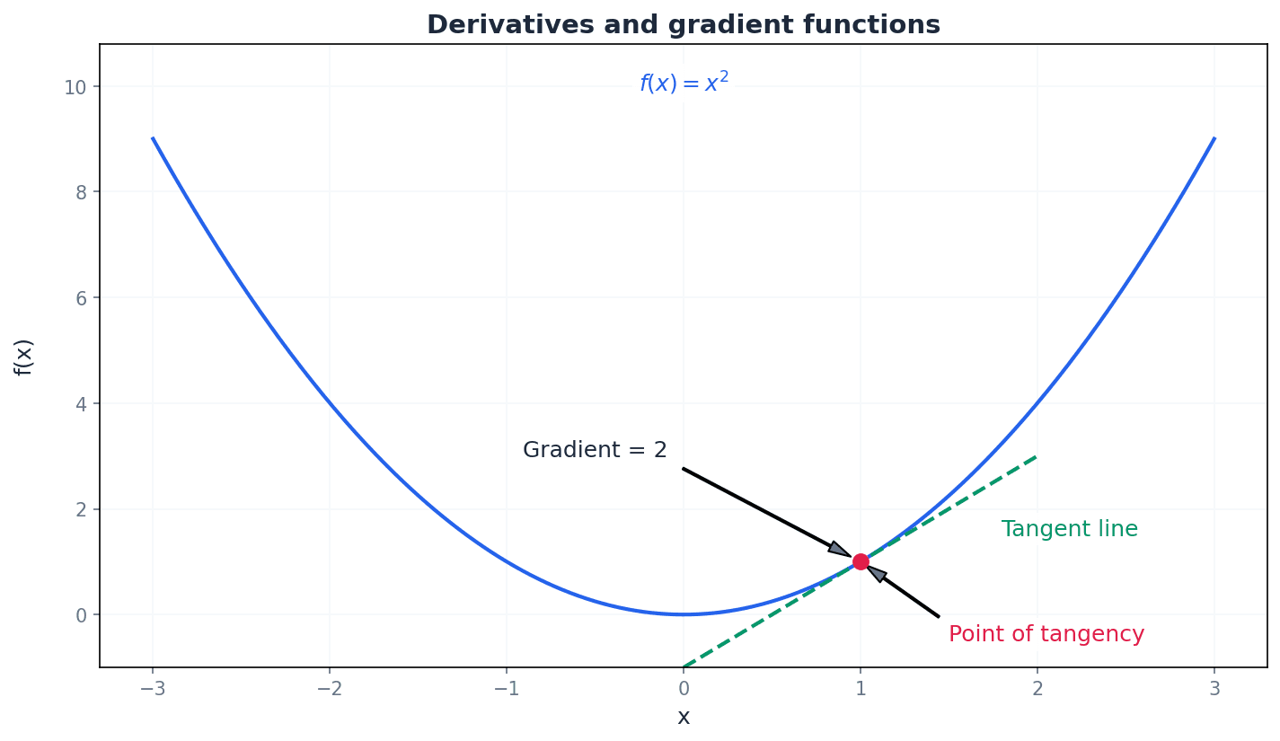
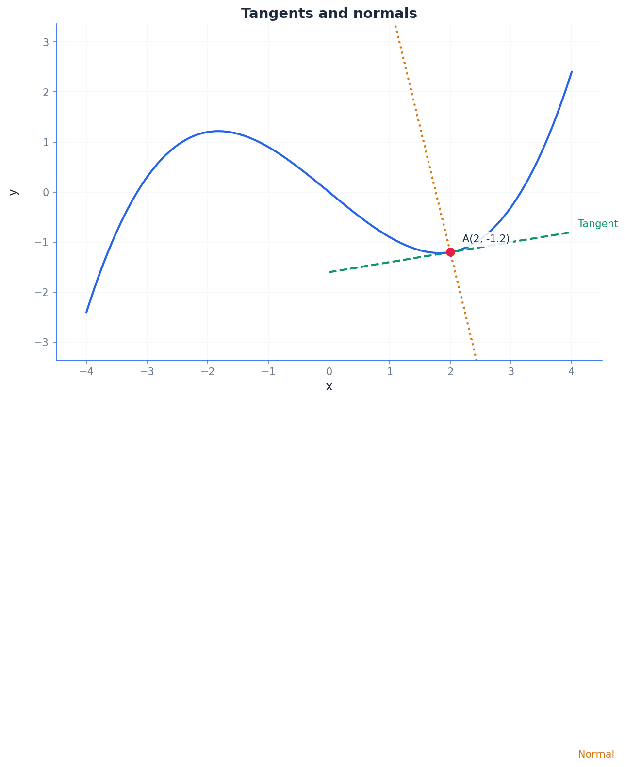
tangent — A straight line that touches a curve at a single point and has the same gradient as the curve at that point.
The equation of the tangent at a point on a curve with gradient is given by . Finding the tangent involves calculating the derivative at the specific point. Imagine a ball rolling along a curved track. If you suddenly remove the track at a certain point, the ball would continue in a straight line along the tangent at that point.
Equation of Tangent
Use the numerical value of the gradient m, not the derivative formula. This formula applies when m is not undefined.
Always calculate the gradient (m) by substituting the x-coordinate into the derivative first, then use the point-gradient formula for the line equation.
Students often think a tangent can never cross the curve, but actually it can cross the curve at other points, especially for more complex functions, as long as it only 'touches' at the point of tangency.
normal — A straight line that is perpendicular to the tangent at a specific point on a curve.
If the gradient of the tangent at a point is , the gradient of the normal at that point is (provided ). The equation of the normal is then found using the point-gradient formula. If the tangent is the direction a ball would fly off a track, the normal is the line pointing directly into or out of the track at that point, like a radius to a circle.
Equation of Normal
This formula applies when m is not zero. If m=0, the tangent is horizontal and the normal is vertical, with equation .
Students often forget to use the negative reciprocal for the normal's gradient, but actually this is crucial for perpendicular lines.
If the tangent is horizontal (m=0), the normal is vertical (x = constant). Be careful not to use the -1/m formula in this case, as it would involve division by zero.
When finding equations of tangents and normals, ensure you have both the gradient (m) and a point (x1, y1). Clearly state the first derivative (dy/dx or f'(x)) before substituting values to find specific gradients.
Practice differentiating various forms of , including fractional and negative powers, to build fluency. Show all steps when applying the chain rule, especially for complex composite functions, to avoid calculation errors.
Exam Technique
Differentiating a function
Finding the gradient of a curve at a point
| Mistake | Fix |
|---|---|
| Confusing the derivative with the original function's value. | Remember the derivative (f'(x) or dy/dx) gives the gradient, not the y-value of the curve. The original function f(x) gives the y-value. |
| Forgetting to apply the chain rule when differentiating composite functions (e.g., $(3x+2)^7$). | Always identify the 'inside' function (u) and the 'outside' function. Differentiate the outside with respect to u, then multiply by the derivative of u with respect to x: $\frac{dy}{dx} = \frac{dy}{du} \times \frac{du}{dx}$. |
| Incorrectly calculating the gradient of the normal by not using the negative reciprocal of the tangent's gradient. | For perpendicular lines, if the tangent's gradient is m, the normal's gradient is $-1/m$. Be careful if m=0 (horizontal tangent), as the normal will be a vertical line $x=x_1$. |
This chapter extends differentiation to analyze function behavior, focusing on identifying increasing and decreasing intervals, and locating and classifying stationary points. It introduces tests for determining the nature of these points and applies differentiation to solve optimization problems and calculate connected rates of change.
increasing function — An increasing function f(x) is one where the f(x) values increase whenever the x value increases, meaning f(a) < f(b) whenever a < b.
For a function to be increasing at a point, its gradient at that point must be positive (dy/dx > 0). If the gradient is positive throughout an interval, the function is increasing over that interval, much like walking uphill where your elevation increases as you move forward.
decreasing function — A decreasing function f(x) is one where the f(x) values decrease whenever the x value increases, meaning f(a) > f(b) whenever a < b.
For a function to be decreasing at a point, its gradient at that point must be negative (dy/dx < 0). If the gradient is negative throughout an interval, the function is decreasing over that interval, similar to walking downhill where your elevation decreases as you move forward.
Students often think an increasing or decreasing function must always have a positive or negative second derivative, respectively. However, the second derivative only tells you about the concavity, not whether the function is increasing or decreasing.
When asked to find the range of values for which a function is increasing, set the first derivative f'(x) > 0 and solve the inequality. Remember to consider the domain of the function.
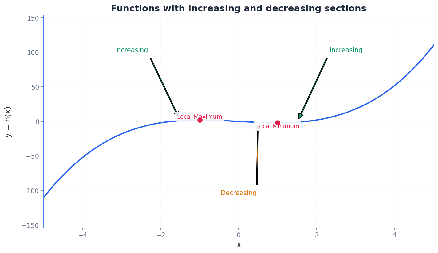
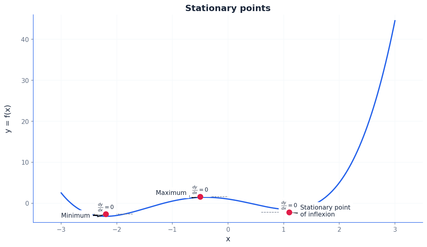
stationary point — A stationary point, also called a turning point, is a point on a curve where the gradient is zero (dy/dx = 0).
At a stationary point, the function momentarily stops increasing or decreasing. These points are crucial for identifying local maximums, minimums, or points of inflexion, representing significant features of a function's graph, much like a ball momentarily stationary at the top of a hill or bottom of a valley.
turning point — A turning point is another name for a stationary point, where the gradient of the curve is zero.
Turning points are where the function changes from increasing to decreasing (a maximum) or from decreasing to increasing (a minimum). They are critical for understanding the shape and behavior of a function's graph, emphasizing the change in the curve's direction.
Students often think all stationary points are either maximums or minimums. However, a stationary point can also be a stationary point of inflexion where the curve flattens out but continues in the same direction.
To find stationary points, always set the first derivative dy/dx = 0 and solve for x. Then substitute these x-values back into the original function to find the corresponding y-coordinates.
maximum points — A maximum point is a stationary point where the value of y is greater than the value of y at other points close to it, and the gradient changes from positive to zero then to negative.
At a maximum point, the curve reaches a 'peak' in its local vicinity. The first derivative is positive to the left, zero at the point, and negative to the right. This is like the summit of a hill, where you go uphill, are momentarily flat, then go downhill.
minimum points — A minimum point is a stationary point where the value of y is less than the value of y at other points close to it, and the gradient changes from negative to zero then to positive.
At a minimum point, the curve reaches a 'trough' in its local vicinity. The first derivative is negative to the left, zero at the point, and positive to the right. This is analogous to the bottom of a valley, where you go downhill, are momentarily flat, then go uphill.
stationary points of inflexion — A stationary point of inflexion is a stationary point where the gradient is zero, but the gradient does not change sign (e.g., positive to zero to positive, or negative to zero to negative).
At a stationary point of inflexion, the curve flattens out momentarily but continues in the same direction. The second derivative at such a point is zero, making the second derivative test inconclusive. This is like a road that briefly levels out on a gentle slope before continuing to slope upwards.
second derivative — The second derivative of y with respect to x, written as d²y/dx², is the rate of change of the gradient (dy/dx) with respect to x.
The second derivative provides information about the concavity of a curve. If d²y/dx² > 0, the curve is concave up (like a valley), indicating a minimum point. If d²y/dx² < 0, the curve is concave down (like a hill), indicating a maximum point. If d²y/dx² = 0, the test is inconclusive, similar to how acceleration describes the rate of change of velocity.
Once stationary points are located by setting dy/dx = 0, their nature (maximum, minimum, or stationary point of inflexion) can be determined using either the first or second derivative test. The first derivative test involves checking the sign of dy/dx on either side of the stationary point. For a maximum, the gradient changes from positive to negative; for a minimum, it changes from negative to positive. For a stationary point of inflexion, the gradient does not change sign.
To confirm a maximum point using the second derivative test, ensure that d²y/dx² < 0 at the stationary point. For a minimum, d²y/dx² > 0. If d²y/dx² = 0, the test is inconclusive, and you must use the first derivative test.
Students often confuse a local maximum with a global maximum, or a local minimum with a global minimum. Remember that a local extremum is only the highest or lowest point in its immediate vicinity, not necessarily on the entire graph.
Differentiation is a powerful tool for solving practical optimization problems where we need to find the maximum or minimum value of a quantity. This often involves setting up an equation for the quantity to be optimized in terms of a single variable, differentiating it, and then finding the stationary points. The nature of these points must then be verified in the context of the problem.
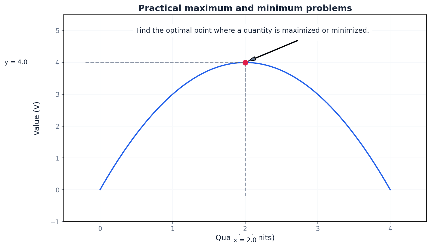
Errors in algebraic manipulation when setting up equations for practical maximum/minimum problems are common. Ensure all variables are correctly defined and relationships are accurately translated into mathematical expressions.
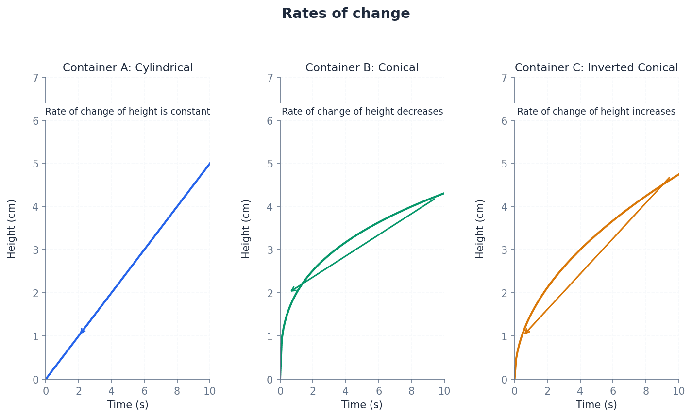
rate of change — The rate of change describes how one quantity changes in relation to another, often with respect to time.
In calculus, the rate of change is represented by the derivative. For example, dy/dx is the rate of change of y with respect to x, and dV/dt is the rate of change of volume with respect to time. These rates can be constant or variable, much like speed is the rate of change of distance with respect to time.
When two variables are related to a third common variable, often time, their rates of change can be connected using the chain rule. This allows us to find an unknown rate of change given other known rates. For instance, if the volume of a sphere is changing with respect to time, and its radius is also changing with respect to time, these rates are connected.
Chain Rule for Connected Rates of Change
Used when two variables (x and y) both vary with a third variable (t) to find the rate of change of y with respect to t.
Chain Rule for Reciprocal Rates
Used to find the rate of change of x with respect to y, given the rate of change of y with respect to x.
Students often incorrectly apply the chain rule for connected rates of change, especially with reciprocal rates or multiple intermediate variables. Carefully identify the variables and their relationships before applying the rule.
For rates of change problems, identify all given rates and the rate to be found, then apply the chain rule correctly, showing all steps.
When sketching graphs, use information about stationary points, intercepts, and asymptotes to ensure accuracy. Clearly show your working for finding dy/dx = 0 and solving for x to locate stationary points.
Exam Technique
Finding increasing/decreasing intervals of a function
Locating and classifying stationary points
| Mistake | Fix |
|---|---|
| Confusing local maximum/minimum with global maximum/minimum. | Always consider the domain of the function and check endpoints if applicable, as a local extremum may not be the absolute highest or lowest point. |
| Incorrectly applying the second derivative test when d²y/dx² = 0. | If d²y/dx² = 0 at a stationary point, the second derivative test is inconclusive. You MUST revert to the first derivative test by checking the sign of dy/dx on either side of the point. |
| Assuming all stationary points are turning points. | Remember that a stationary point can also be a stationary point of inflexion, where the gradient is zero but does not change sign. |
This chapter introduces integration as the reverse process of differentiation, covering both indefinite and definite integrals. It explains how to find the constant of integration and apply integration to calculate areas bounded by curves and lines, as well as volumes of revolution. The concept of improper integrals for unbounded regions or functions is also discussed.
antidifferentiation — The reverse process of differentiation.
Antidifferentiation is the process of finding a function given its derivative. This process is essentially what integration achieves, and due to the Fundamental Theorem of Calculus, it is equivalent to finding the area under a curve. If differentiation is like finding the rate of change of a quantity, antidifferentiation is like finding the original quantity given its rate of change.
indefinite integral — An integral without limits whose result contains a constant of integration.
When you integrate a function, you are finding a family of functions whose derivative is the original function. Since the derivative of a constant is zero, there are infinitely many such functions, differing only by a constant 'c'. This 'c' is the constant of integration. Imagine you know the speed of a car at every moment, and you want to find its position. You can find its change in position, but without knowing its starting position, you can't know its exact final position. The starting position is like the constant of integration.
constant of integration — An arbitrary constant added to the result of indefinite integration.
When a function is differentiated, any constant term disappears. Therefore, when reversing the process (integrating), there's an unknown constant that could have been present in the original function. This constant, 'c', represents that unknown value. If you know that someone's age increased by 5 years, you don't know their current age unless you know their age 5 years ago. The 'age 5 years ago' is like the constant of integration.
Students often forget to add the constant of integration '+ c' when performing indefinite integration. Always remember to add '+ c' when performing indefinite integration. Failure to do so is a common error and will result in loss of marks.
Students may incorrectly assume that the constant of integration 'c' is always zero, leading to incorrect curve equations. The constant of integration 'c' can be any real number and is determined by additional information (like a point on the curve).
Always remember to add '+ c' when performing indefinite integration. Failure to do so is a common error and will result in loss of marks.
Power Rule for Integration
Valid for any rational n except n = -1.
Integration of Constant Multiple
The constant k can be factored out of the integral.
Integration of Sums and Differences
Integration can be applied term by term to sums and differences of functions.
Integration of (ax + b)^n
Valid for n \neq -1 and for powers of linear functions only.
Integration is fundamentally the reverse process of differentiation, also known as antidifferentiation. When we differentiate a function, we find its rate of change. Conversely, when we integrate, we are finding the original function given its rate of change. This process allows us to move from a derivative back to the original function, though it introduces an unknown constant.
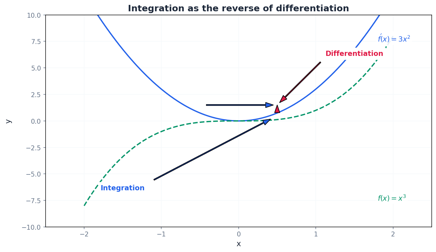
Since the derivative of any constant is zero, when we integrate, there is always an arbitrary constant 'c' that could have been present in the original function. To find the specific value of this constant, additional information is required, typically a point that lies on the curve. By substituting the coordinates of this point into the integrated equation, we can solve for 'c' and determine the unique equation of the curve.
Problems involving finding the constant of integration usually provide a point on the curve. Substitute the coordinates of this point into the integrated equation to solve for 'c'.
definite integral — An integral between limits whose result does not contain a constant of integration.
Definite integrals are used to find the exact value of the area under a curve between two specific points, known as the limits of integration. The constant of integration cancels out when evaluating the integral at the upper and lower limits. If an indefinite integral is like finding all possible paths a car could take, a definite integral is like finding the exact distance the car travelled between two specific times.
limits of integration — The specified values between which a function is integrated.
These are the upper and lower bounds of the interval over which the definite integral is calculated. They define the specific region for which the area or volume is being determined. If you're measuring the length of a segment of road, the limits of integration are like the start and end markers of that segment.
Students often think that definite integrals still require a '+ c', but actually the constant of integration cancels out during the evaluation process.
When evaluating definite integrals, ensure you substitute the upper limit first, then the lower limit, and subtract the results. Pay close attention to signs, especially with negative values.
Evaluation of Definite Integral
The constant of integration 'c' cancels out in definite integrals.
Definite Integral of Constant Multiple
The constant k can be factored out of a definite integral.
Definite Integral of Sums and Differences
Definite integration can be applied term by term to sums and differences.
Definite Integral Property (Splitting Interval)
The point 'c' must be between 'a' and 'b'.
Fundamental theorem of Calculus — A theorem stating that integration is essentially the same as antidifferentiation.
This theorem establishes a crucial link between the two main branches of calculus: differentiation and integration. It shows that the process of finding the area under a curve is directly related to finding the antiderivative of the function. It's like discovering that unlocking a door is the exact reverse process of locking it, even if they seem like different actions at first glance.
Definite integration is a powerful tool for calculating the area of a region bounded by a curve and lines. The integral \(\int_a^b f(x) \, dx\) represents the area between the curve \(y = f(x)\), the x-axis, and the vertical lines \(x=a\) and \(x=b\). If the curve lies below the x-axis, the integral will yield a negative value, so the absolute value must be taken to represent the area. Similarly, for areas bounded by the y-axis, we integrate with respect to y.
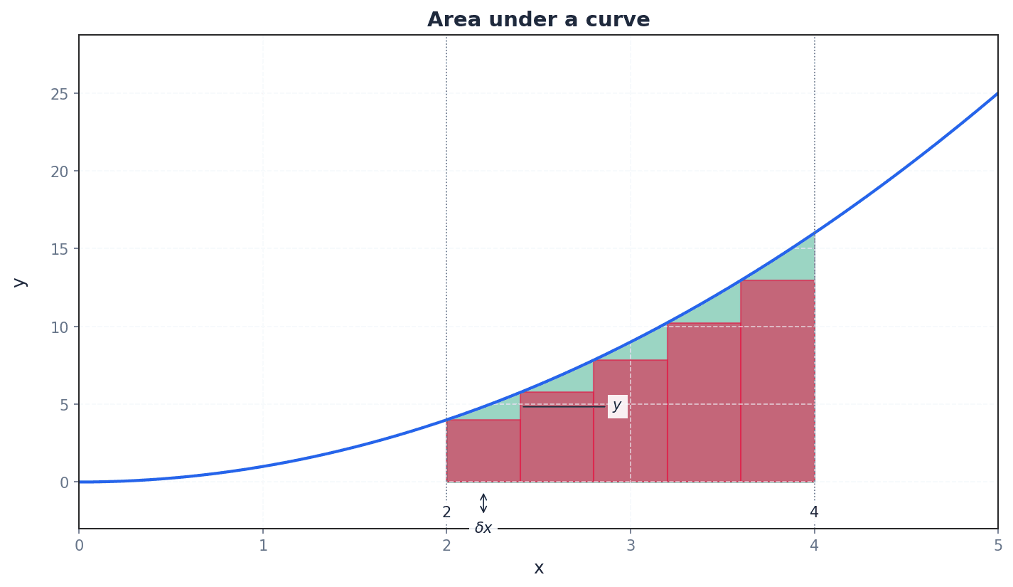
Area under a curve (x-axis)
If the curve is below the x-axis, the integral will be negative, so take the absolute value for area.
Area under a curve (y-axis)
Used when the curve is defined as x = f(y) and bounded by the y-axis and horizontal lines y=a and y=b.
To find the area enclosed between two curves, \(y = f(x)\) and \(y = g(x)\), over an interval from \(x=a\) to \(x=b\), we integrate the difference between the upper function and the lower function. The formula is \(A = \int_a^b [f(x) - g(x)] \, dx\), where \(f(x)\) is the upper curve and \(g(x)\) is the lower curve in the specified interval. The limits of integration, \(a\) and \(b\), are often the x-coordinates of the intersection points of the two curves.
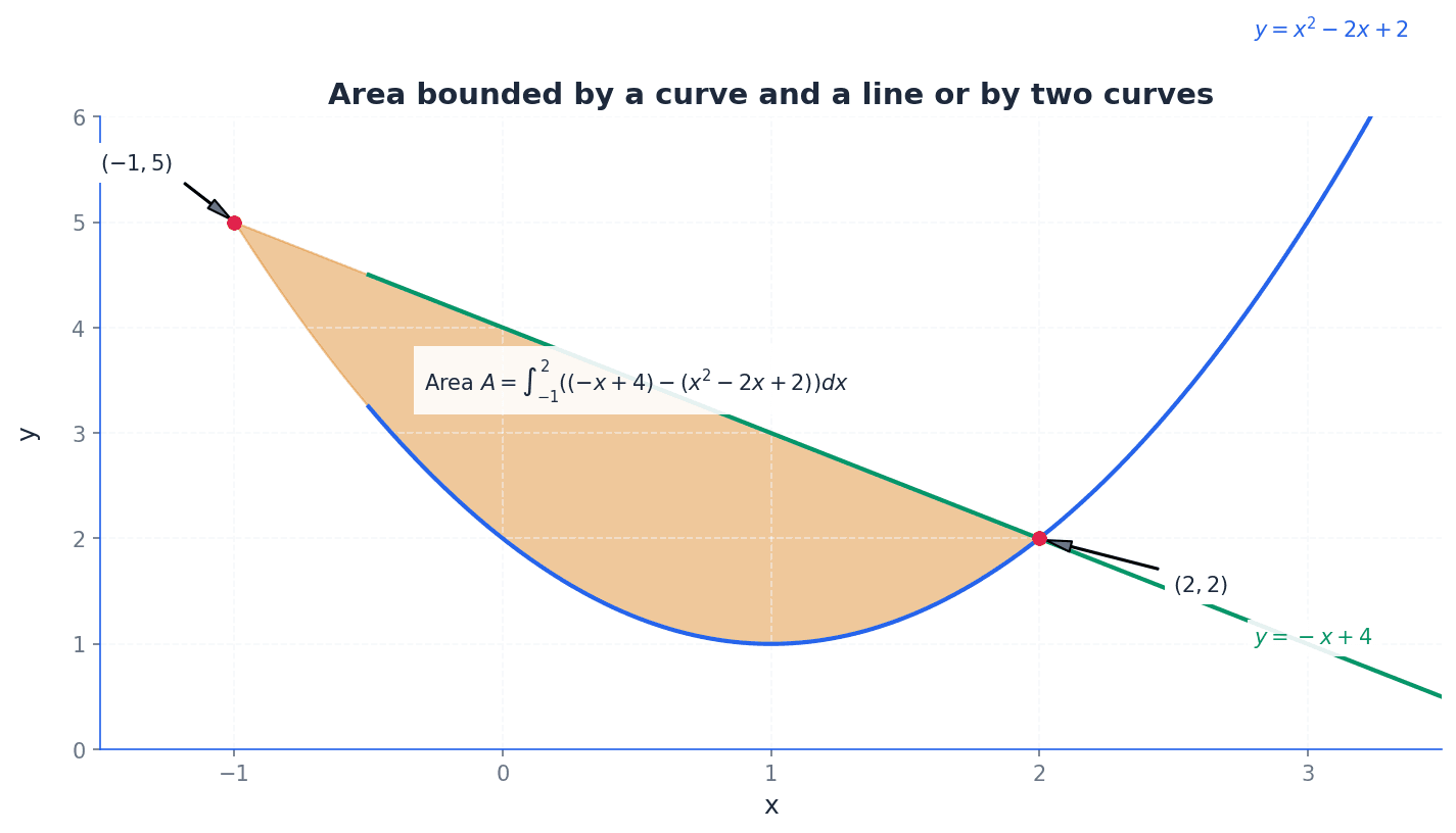
Area between two curves
f(x) must be greater than or equal to g(x) over the interval [a, b].
When calculating area, students might get a negative result if the region is below the x-axis and forget to take the absolute value. Always take the absolute value for area if the integral yields a negative result.
solid of revolution — A three-dimensional solid formed when an area is rotated through 360 degrees about an axis.
This concept allows us to calculate the volume of complex 3D shapes by integrating the volumes of infinitesimally thin discs or washers formed by rotating small segments of the 2D area. Imagine spinning a flat cardboard cutout of a shape very fast around a stick; the blurred 3D shape you see is a solid of revolution.
volume of revolution — The volume of the solid formed when an area is rotated through 360 degrees about an axis.
This is the quantitative measure of the space occupied by a solid of revolution. It is calculated using definite integration, summing the volumes of infinitesimally thin cylindrical discs or washers. It's like calculating how much clay is needed to make a vase by spinning a profile shape on a potter's wheel.
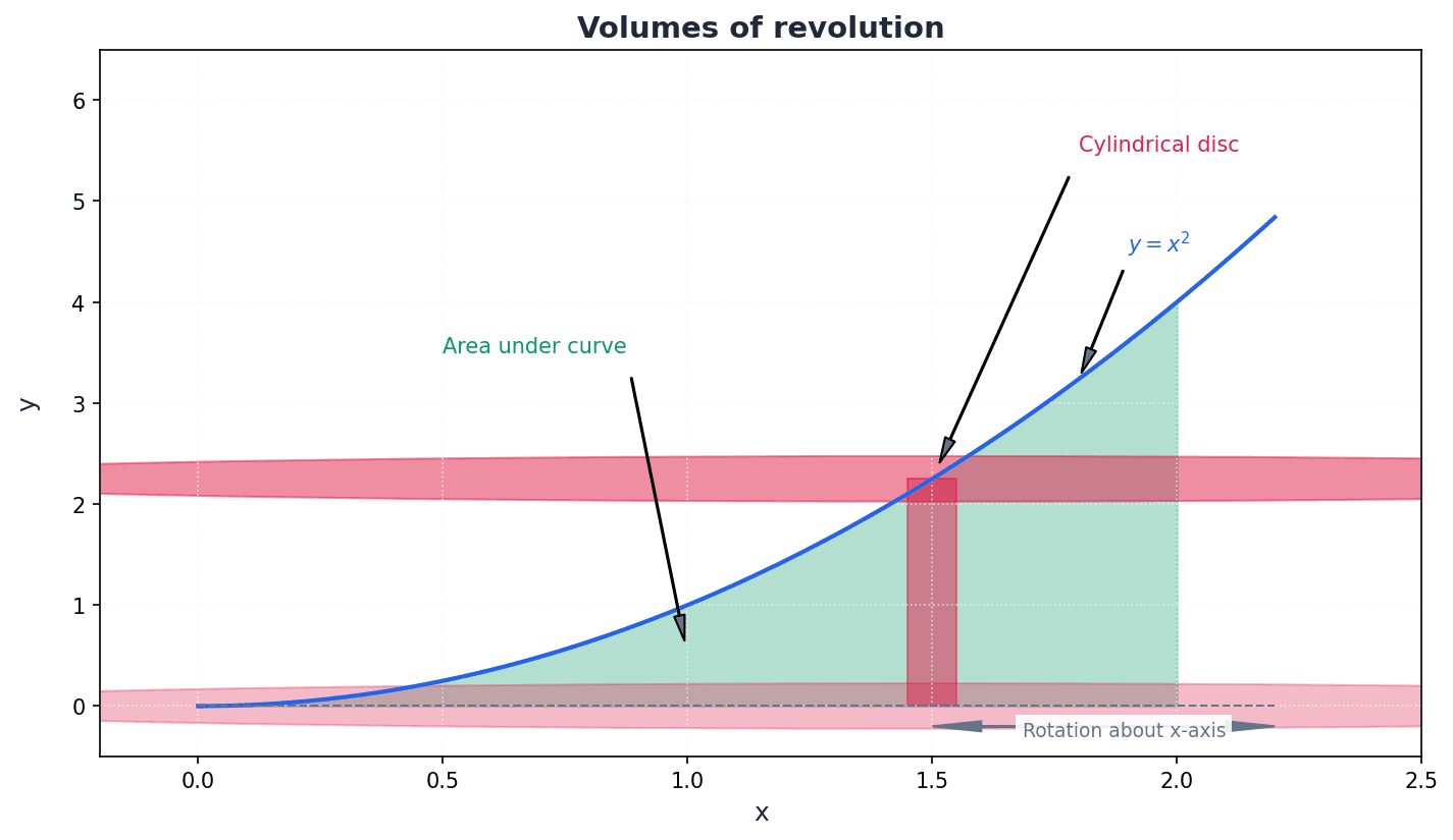
Volume of Revolution (about x-axis)
Used when rotating a function y = f(x) about the x-axis.
Volume of Revolution (about y-axis)
Used when rotating a function x = f(y) about the y-axis.
When calculating volumes of revolution, students often forget to square the function (y or x) or omit the factor of \(\pi\) in the formula. Always include \(\pi\) and square the radius in your volume of revolution calculations.
Students sometimes confuse the axis of rotation (x-axis vs. y-axis) and use the wrong variable of integration or formula for volume of revolution. Carefully identify the axis of rotation as this determines whether you integrate with respect to x or y, and whether the radius is y or x.
Always include \(\pi\) in your volume of revolution calculations. If the region has a 'hole' (e.g., rotating an area between two curves), remember to subtract the volume of the inner solid from the volume of the outer solid.
improper integrals — Definite integrals where either one or both limits are infinite, or where the function to be integrated approaches an infinite value at either or both endpoints in the interval.
These integrals extend the concept of definite integration to cases where the interval of integration is unbounded or the function itself becomes unbounded within the interval. They are evaluated by taking limits. Imagine trying to find the total amount of sand in a desert that stretches infinitely in one direction, or the total volume of water in a funnel that gets infinitely narrow at its tip.
For improper integrals, students might incorrectly assume that all integrals with infinite limits or discontinuities diverge (tend to infinity), when many actually converge to a finite value. Many improper integrals converge to a finite value, so always evaluate by taking limits.
When evaluating improper integrals, always replace the infinite limit or the point of discontinuity with a variable (e.g., X) and then take the limit as that variable approaches the problematic value. Show all limit notation clearly.
Always show your working for finding the constant of integration, even if it's zero. When calculating areas, sketch the graph to identify regions above and below the x-axis, and determine correct limits. For volumes of revolution, clearly state the formula you are using and the limits of integration. Pay close attention to the limits of integration for definite integrals; a small error can lead to a completely wrong answer. If an improper integral is given, remember to use limits and evaluate the integral as a limit.
Exam Technique
Indefinite Integration of Power Functions
Finding the Equation of a Curve from its Gradient Function
| Mistake | Fix |
|---|---|
| Forgetting to add '+ c' for indefinite integrals. | Always include '+ c' in your final answer for indefinite integrals. This is a fundamental part of the definition. |
| Assuming 'c' is always zero when finding the equation of a curve. | Use any given point on the curve to substitute x and y values into the integrated equation and solve for 'c'. 'c' is rarely zero unless specified. |
| Incorrectly evaluating definite integrals (e.g., \(F(a) - F(b)\) instead of \(F(b) - F(a)\)). | Always substitute the upper limit first, then the lower limit, and subtract the lower from the upper: \(F(b) - F(a)\). Pay close attention to signs. |
Generated by Nexelia Academy · nexeliaacademy.com