Nexelia Academy · Official Revision Notes
Complete A-Level revision notes · 11 chapters
This chapter covers the modulus function, including its definition, graphical representation, and methods for solving related equations and inequalities. It also introduces polynomial division, the factor theorem, and the remainder theorem, which are essential tools for factorising and solving cubic and quartic polynomial equations.
modulus — The modulus of a number is the magnitude of the number without a sign attached.
Also known as the absolute value, the modulus of any number (positive or negative) is always a positive number. For example, the modulus of 3 is 3, and the modulus of -3 is also 3. Think of the modulus as the 'distance from zero' on a number line. Whether you go 3 units to the right (positive) or 3 units to the left (negative), the distance covered is always 3 units.
absolute value — The modulus of a number is also called the absolute value.
This term is synonymous with 'modulus' and refers to the non-negative numerical value of a number, disregarding its sign. It is commonly denoted by vertical bars, e.g., |x|. If you're measuring the length of something, you always get a positive value, regardless of its orientation. The absolute value is like that 'length' of a number.
polynomial — A polynomial is an expression of the form a_n x^n + a_{n-1} x^{n-1} + … + a_1 x + a_0, where x is a variable, n is a non-negative integer, the coefficients a_0, a_1, ..., a_n are constants, a_n is called the leading coefficient and a_n ≠ 0, and a_0 is called the constant term.
Polynomials are fundamental algebraic expressions built from variables and coefficients using only addition, subtraction, multiplication, and non-negative integer exponents of the variable. The highest power of x in the polynomial determines its degree. Think of a polynomial as a 'recipe' for a function, where you combine different powers of x (like different ingredients) with specific constant amounts (coefficients) to create a mathematical expression.
leading coefficient — In a polynomial a_n x^n + a_{n-1} x^{n-1} + … + a_1 x + a_0, a_n is called the leading coefficient and a_n ≠ 0.
The leading coefficient is the coefficient of the term with the highest degree in a polynomial. It plays a crucial role in determining the end behaviour of the polynomial's graph. In a race, the 'leading runner' is the one at the front. Similarly, the leading coefficient is the number 'in front' of the highest power of x in a polynomial.
constant term — In a polynomial a_n x^n + a_{n-1} x^{n-1} + … + a_1 x + a_0, a_0 is called the constant term.
The constant term in a polynomial is the term that does not contain any variable, essentially the coefficient of x^0. It represents the y-intercept of the polynomial's graph. It's like the 'base cost' in a pricing formula – it's a fixed value that doesn't change regardless of the quantity (x) you buy.
degree of the polynomial — The highest power of x in the polynomial is called the degree of the polynomial.
The degree of a polynomial is a non-negative integer that indicates the highest exponent of the variable in any term of the polynomial. It helps classify polynomials (e.g., linear, quadratic, cubic) and influences the number of roots and the shape of its graph. Think of the degree as the 'level' of the polynomial. A higher degree means a more complex shape for its graph, just like a higher level in a game means more complexity.
dividend — In polynomial division, the dividend is the polynomial being divided.
When performing algebraic long division, the dividend is the polynomial that is 'inside' the division symbol. It is expressed as dividend = divisor × quotient + remainder. If you're sharing a cake, the whole cake is the dividend – it's what's being divided among people.
divisor — In polynomial division, the divisor is the polynomial by which another polynomial is divided.
The divisor is the polynomial that 'divides into' the dividend. If the remainder is zero, the divisor is a factor of the dividend. Continuing the cake analogy, the divisor is the number of people you're sharing the cake with – it's what you're dividing by.
quotient — In polynomial division, the quotient is the result of the division, excluding any remainder.
The quotient is the polynomial obtained when the dividend is divided by the divisor. It represents how many times the divisor 'fits into' the dividend. If you divide 10 by 3, the quotient is 3 – it's the whole number result of the division.
remainder — In polynomial division, the remainder is the polynomial left over after the division process, which has a degree less than the divisor.
The remainder is what is 'left over' after dividing one polynomial by another. If the remainder is zero, the divisor is a factor of the dividend. The remainder theorem provides a shortcut to find this value for linear divisors. If you divide 10 by 3, the remainder is 1 – it's what's left over after you've taken out as many whole groups of 3 as possible.
factor — If a polynomial P(x) divides exactly by a linear factor (x - c) to give the polynomial Q(x), then (x - c) is a factor of P(x).
A factor of a polynomial is an expression that divides the polynomial evenly, resulting in a remainder of zero. The factor theorem provides a direct way to test if a linear expression is a factor. In numbers, 2 is a factor of 6 because 6 divided by 2 leaves no remainder. Similarly, in polynomials, a factor divides without leaving a remainder.
factor theorem — If for a polynomial P(x), P(c) = 0, then (x - c) is a factor of P(x).
This theorem provides a quick method to determine if a linear expression (x - c) is a factor of a polynomial P(x) by simply evaluating P(x) at x = c. If the result is zero, then (x - c) is a factor. It's like a 'key test' for a lock. If you put the key (c) into the lock (P(x)) and it 'opens' (equals zero), then that key is a factor of the lock.
remainder theorem — If a polynomial P(x) is divided by (x - c), the remainder is P(c).
This theorem states that when a polynomial P(x) is divided by a linear divisor (x - c), the remainder of that division is equal to the value of the polynomial when x is replaced by c. It's a generalization of the factor theorem. Imagine you're trying to guess how much 'leftover' you'll have after sharing. The remainder theorem tells you that if you just 'try out' the sharing amount (c) in the original recipe (P(x)), you'll get the leftover directly.
x-intercept — The x-intercept is the point where the graph meets the x-axis.
At the x-intercept, the y-coordinate of the point is always zero. For a function y = f(x), the x-intercepts are the solutions to the equation f(x) = 0, also known as the roots of the equation. Imagine a car driving across a road. The x-intercept is where the car crosses the main road (the x-axis).
y-intercept — The y-intercept is the point where the graph meets the y-axis.
At the y-intercept, the x-coordinate of the point is always zero. For a function y = f(x), the y-intercept is found by evaluating f(0). Continuing the car analogy, the y-intercept is where the car crosses a side road (the y-axis).
vertex — The vertex of a modulus function graph of the form y = |ax + b| is the point where the graph changes direction, forming a 'V' shape.
For a modulus function y = |f(x)|, the vertex occurs where f(x) = 0. This is the point where the reflection in the x-axis takes place, resulting in the sharp turn of the graph. Think of the vertex as the 'hinge' of a folding ruler. It's the point where the two parts of the graph meet and change direction.
intersection — An intersection point is a point where two or more graphs meet.
The coordinates of an intersection point satisfy the equations of all the graphs that pass through it. Finding intersection points is a common method for solving simultaneous equations or inequalities graphically. Imagine two roads crossing each other. The point where they cross is their intersection.
inequality — An inequality is a mathematical statement that compares two expressions using an inequality symbol (e.g., <, >, ≤, ≥).
Solving an inequality means finding the range of values for the variable that makes the statement true. For modulus inequalities, this often involves considering different cases or interpreting graphs. Think of an inequality as setting a 'boundary' or a 'limit'. For example, x > 5 means x must be greater than 5, not just equal to it.
Modulus of x
Defines the modulus (absolute value) of a number.
Modulus equation property 1
Used to solve equations of the form |ax + b| = c, where 'a' is a positive constant.
Modulus equation property 2
Used to solve equations of the form |ax + b| = |cx + d|. This can also be written as ax + b = ±(cx + d).
Modulus inequality property 1
Used to solve modulus inequalities where the modulus is less than a positive constant.
Modulus inequality property 2
Used to solve modulus inequalities where the modulus is greater than a positive constant.
Division algorithm for polynomials
Relates the dividend P(x), divisor D(x), quotient Q(x), and remainder R(x) in polynomial division. The degree of the remainder R(x) must be less than the degree of the divisor D(x).
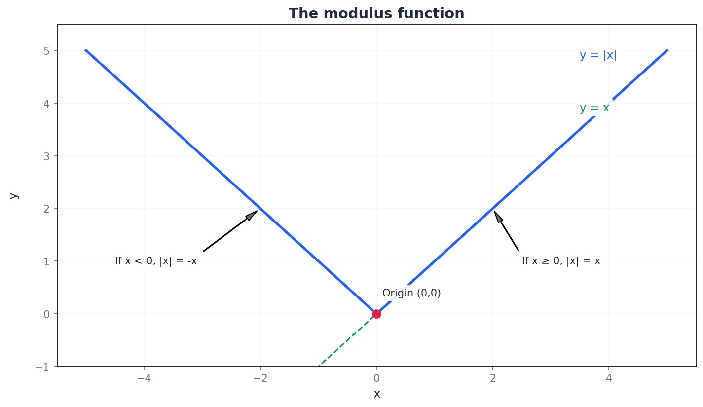
The modulus function, also known as the absolute value, gives the magnitude of a number without its sign. It is defined as |x| = x if x ≥ 0, and |x| = -x if x < 0. This means the output of a modulus function is always a non-negative value. For example, |3| = 3 and |-3| = 3.
Students often think that |x| can be negative, but actually the modulus function always returns a non-negative value.
To solve equations involving the modulus function, such as |ax + b| = c, we consider two cases: ax + b = c or ax + b = -c. For equations of the form |ax + b| = |cx + d|, squaring both sides, i.e., (ax + b)^2 = (cx + d)^2, is an effective method. It is crucial to check all solutions in the original equation, especially when squaring, as extraneous roots can arise.
When solving equations or inequalities involving modulus, remember to consider both the positive and negative cases of the expression inside the modulus. For example, |x| = a means x = a or x = -a.
Students often forget to check solutions for modulus equations of the form |ax + b| = cx + d, as extraneous roots can arise from squaring both sides.
The graph of a modulus function of the form y = |ax + b| or y = |f(x)| where f(x) is linear, forms a characteristic 'V' shape. This shape is created by reflecting the part of the graph of y = f(x) that lies below the x-axis, upwards across the x-axis. The vertex of this 'V' shape is located at the x-intercept of the original linear function, i.e., where ax + b = 0.
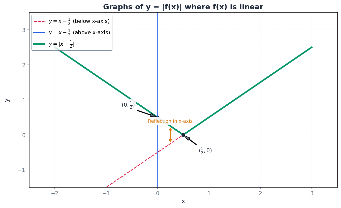
When sketching modulus graphs, accurately identifying and labelling the coordinates of the vertex is crucial for demonstrating understanding. Also, clearly label the coordinates of all x-intercepts and the y-intercept.
Students often think the vertex is always at the origin, but actually it depends on the linear function inside the modulus, i.e., where ax + b = 0.
Modulus inequalities can be solved algebraically by applying specific properties. For |x| < a, the solution is -a < x < a. For |x| > a, the solution is x < -a or x > a. Alternatively, graphical interpretation can be used by sketching the graphs of the functions involved and identifying the regions where the inequality holds true. Always check your solutions by substituting values from the determined range back into the original inequality.
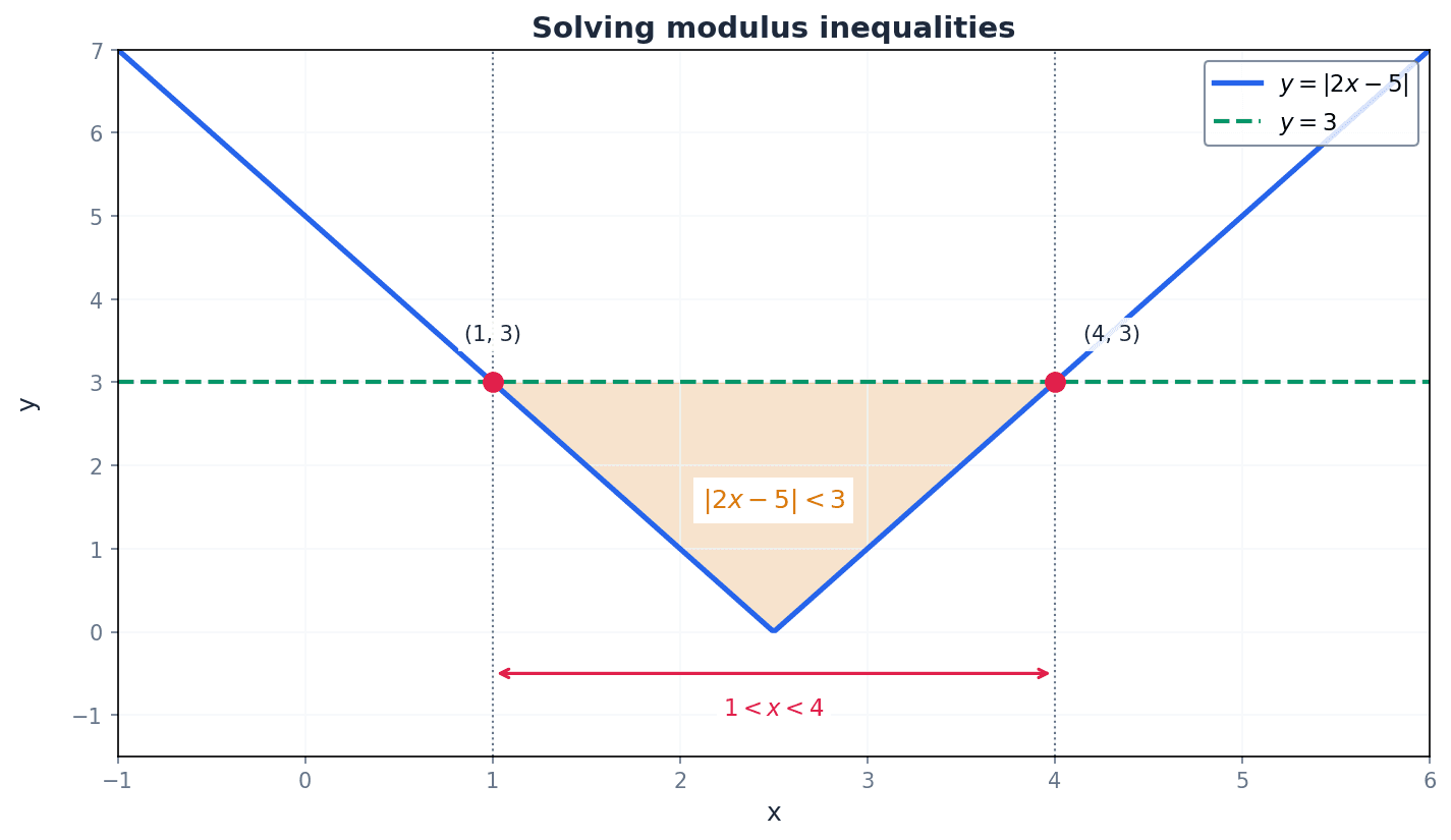
Students often confuse the conditions for modulus inequalities, e.g., using |x| > a for |x| < a, or vice versa. Remember that |x| < a means 'between' (-a < x < a), while |x| > a means 'outside' (x < -a or x > a).
Students often forget to reverse the inequality sign when multiplying or dividing by a negative number in algebraic manipulation.
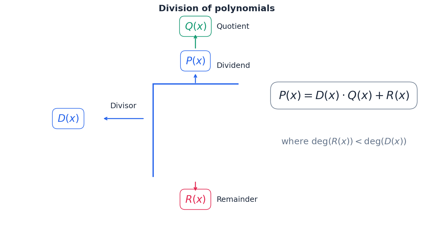
Polynomial division is a method for dividing a polynomial (the dividend) by another polynomial (the divisor) to find a quotient and a remainder. The division algorithm for polynomials states P(x) = D(x)Q(x) + R(x), where the degree of the remainder R(x) must be less than the degree of the divisor D(x). This process is similar to numerical long division and is crucial for factorising and solving higher-degree polynomial equations.
Ensure you write the dividend in descending powers of x, including zero coefficients for any missing terms, to avoid errors in long division.
Students often forget to include zero coefficients for missing terms when performing polynomial long division, leading to incorrect alignment and calculations.
The Factor Theorem is a powerful tool stating that if P(c) = 0 for a polynomial P(x), then (x - c) is a factor of P(x). This allows for quick identification of linear factors. The Remainder Theorem generalizes this, stating that when a polynomial P(x) is divided by (x - c), the remainder is P(c). These theorems are invaluable for factorising and solving cubic and quartic polynomial equations by finding initial factors and reducing the polynomial to a quadratic.
The remainder theorem is a powerful tool for quickly finding the remainder when dividing by a linear factor (x - c) without performing full long division.
Students often confuse the factor theorem and the remainder theorem, or apply them incorrectly (e.g., testing P(c) for a factor (ax - b)). Remember the factor theorem is a special case of the remainder theorem where the remainder is zero.
For cubic and quartic equations, use the Factor Theorem to find initial factors, then use algebraic division or equating coefficients to find the remaining factors.
Students often fail to completely factorise polynomials, leaving quadratic factors that could be further broken down.
For modulus equations and inequalities, always consider both algebraic methods (squaring, definition) and graphical interpretation to verify solutions.
Exam Technique
Solve |ax + b| = c
Solve |ax + b| = |cx + d|
| Mistake | Fix |
|---|---|
| Forgetting to consider both positive and negative cases when solving modulus equations or inequalities. | Always split modulus equations/inequalities into two distinct cases based on the definition of modulus, or by squaring both sides carefully. |
| Failing to check for extraneous roots when solving modulus equations of the form |ax + b| = cx + d by squaring. | After solving, substitute all potential solutions back into the original equation. Reject any solution that makes the right-hand side (cx + d) negative, as a modulus cannot equal a negative value. |
| Confusing the conditions for modulus inequalities (e.g., using |x| > a for |x| < a). | Remember: |x| < a means -a < x < a (values 'between'), and |x| > a means x < -a or x > a (values 'outside'). Visualise on a number line or graph if unsure. |
This chapter explores logarithmic and exponential functions, their inverse relationship, and their graphs. It covers the laws of logarithms for any base, including natural logarithms, and their application in solving various equations and inequalities. A key skill is transforming non-linear relationships into linear form using logarithms to determine unknown constants from experimental data.
logarithmic function — A logarithmic function is the inverse of an exponential function.
Logarithmic functions allow us to solve exponential equations where the unknown is in the index. If an exponential function is like asking 'What is 2 to the power of 3?', a logarithmic function is like asking 'To what power must 2 be raised to get 8?'.
logarithm — log10 y is the power that 10 must be raised to in order to obtain y.
This definition applies to any base 'a', where log_a y is the power 'a' must be raised to to obtain 'y'. It is a fundamental concept for solving exponential equations. Think of a logarithm as the 'question' that asks 'What exponent do I need?' for a given base and result.
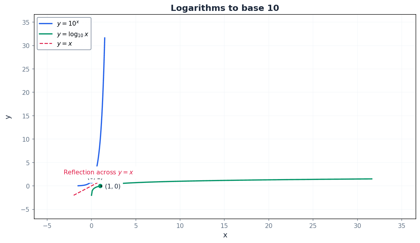
inverse functions — We say that y = 10^x and x = log10 y are inverse functions.
Inverse functions 'undo' each other. If you apply a function and then its inverse, you get back to the original input. Graphically, inverse functions are reflections of each other across the line y = x. Like putting on your shoes (function) and then taking them off (inverse function) – you end up back where you started.
When asked to define a logarithmic function, ensure you explicitly state its relationship as the inverse of an exponential function.
Logarithm Definition (Base 10)
Relates exponential and logarithmic forms for base 10.
Logarithm Definition (General Base)
General definition of a logarithm to base a. y must be positive, and the base 'a' must be positive and not equal to 1.
Logarithm of 1
Any base raised to the power of 0 is 1.
Logarithm of Base
Any base raised to the power of 1 is itself.
Logarithms provide a way to express exponential relationships in an inverse form. The expression means that 'a' raised to the power 'x' equals 'y'. The equivalent logarithmic form, , asks 'to what power must 'a' be raised to obtain 'y'?' This fundamental relationship is crucial for solving equations where the unknown is in the index.
Students often think log_a y means 'a multiplied by y', but actually it means 'the power to which a must be raised to get y'.
Be precise with the base of the logarithm; log 6 (base 10) is different from log_2 6.
Multiplication Law of Logarithms
Used to combine or separate logarithms of products, where x and y must be positive numbers.
Division Law of Logarithms
Used to combine or separate logarithms of quotients, where x and y must be positive numbers.
Power Law of Logarithms
Used to bring exponents out of or into a logarithm, where x must be a positive number and p is any real number.
Special Case of Power Law
Derived from the power law where p = -1, for a positive number x.
The laws of logarithms are essential for simplifying expressions and solving equations. The multiplication law allows us to combine the logarithm of a product into a sum of logarithms, while the division law handles quotients. The power law is particularly useful for bringing down exponents, which is key when solving exponential equations where the unknown is in the index.
Students may incorrectly apply logarithm laws, such as thinking log(x+y) = log x + log y. Remember that the laws only apply to products, quotients, and powers.
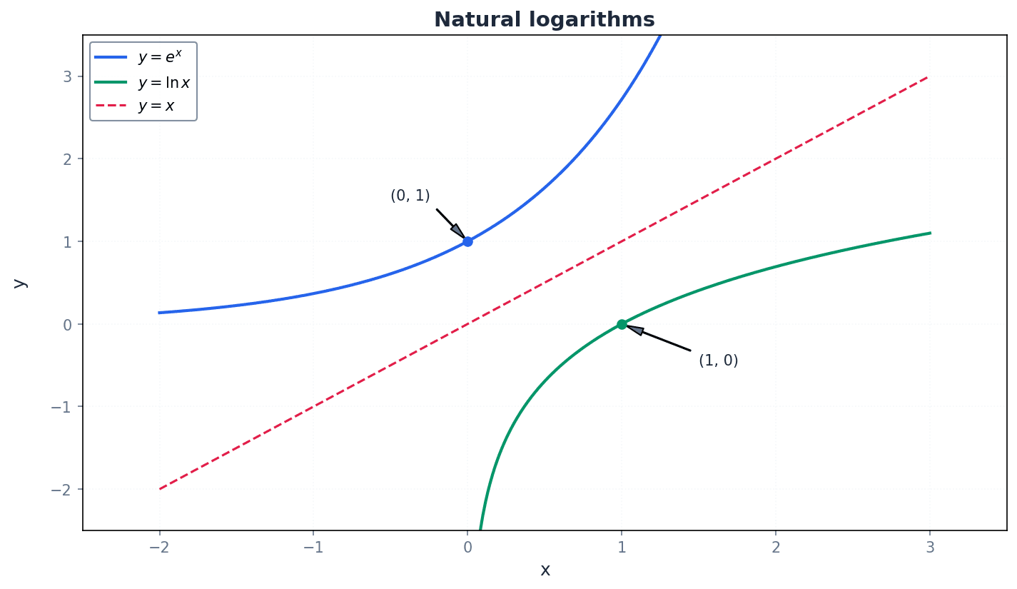
natural exponential function — The function e^x is called the natural exponential function.
This function uses the special irrational number 'e' (approximately 2.718) as its base. It has unique properties in calculus and models continuous growth and decay. If 10^x is like compound interest calculated annually, e^x is like compound interest calculated continuously, growing smoothly at every instant.
natural logarithms — Logarithms to the base of e are called natural logarithms.
Represented as ln x, natural logarithms are the inverse of the natural exponential function e^x. They follow all the same laws of logarithms but are particularly important in calculus and continuous processes. If log10 is like counting in powers of 10, ln is like counting in powers of 'e', which is the natural rate of growth.
Natural Logarithm Definition
Relates natural exponential and natural logarithmic forms.
Remember that e^x is always positive, which is important when solving equations or inequalities involving it.
Students often confuse e^x with 10^x, but actually e is a specific irrational number, not a variable base.
Students often forget that ln x is just log_e x and that all logarithm rules still apply, but actually it's a specific base logarithm with its own notation.
Logarithms are indispensable for solving equations where the unknown appears in the index. By taking the logarithm of both sides, the power law can be used to bring the unknown down, allowing for algebraic manipulation. When solving inequalities, it is crucial to remember that multiplying or dividing by a negative logarithm (e.g., log 0.6) requires reversing the inequality sign.
Students often forget that logarithms are only defined for positive arguments (e.g., log x requires x > 0). Always check for extraneous roots when solving logarithmic equations.
When solving exponential inequalities, students often forget to reverse the inequality sign when dividing by a negative logarithm (e.g., log 0.6 is negative).
When solving equations involving ln x, remember that ln x is only defined for x > 0, so check for extraneous roots.
linear form — Logarithms can be used to convert some curves into straight lines, which is called transforming to linear form.
This technique allows non-linear relationships (like y = kx^n or y = ka^x) to be analysed using straight-line graph properties (gradient and y-intercept). This is useful for determining unknown constants from experimental data. It's like putting on special glasses that make a curvy road look straight, so you can easily measure its slope and where it starts.
gradient — In the linear equation Y = mX + c, m is the gradient.
The gradient represents the rate of change of Y with respect to X. When transforming non-linear equations, the gradient of the resulting straight line can be used to determine one of the unknown constants. The gradient is like the steepness of a hill; a higher gradient means a steeper hill.
y-intercept — In the linear equation Y = mX + c, c is the y-intercept.
The y-intercept is the point where the straight line crosses the Y-axis (i.e., when X = 0). In transformed equations, the y-intercept can be used to determine another unknown constant. The y-intercept is like the starting height of a ramp before it begins to slope upwards.
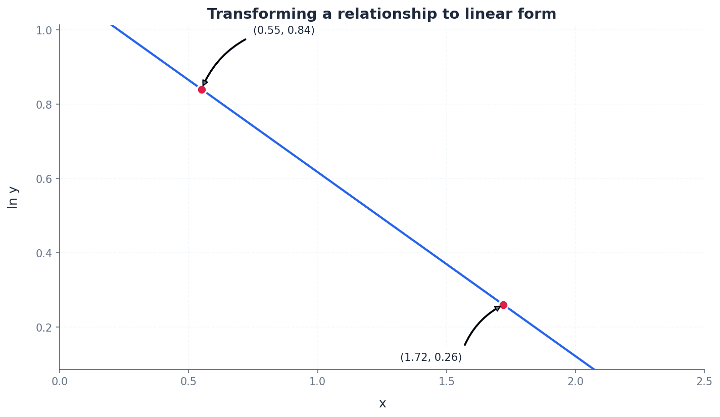
Many real-world relationships are non-linear but can be made linear by applying logarithms. For example, equations like or can be transformed into the form . This allows experimental data to be plotted on a straight-line graph, where the gradient () and y-intercept () can be used to find the unknown constants (, , or ). This is a powerful tool for data analysis.
Students often confuse the original variables (x, y) with the transformed variables (X, Y) in the linear equation Y = mX + c, but actually X and Y must contain only the original variables, not the unknown constants.
Clearly state what X, Y, m, and c represent in terms of the original variables and constants when transforming an equation to linear form.
When sketching graphs of inverse functions, always include the line y = x to show the reflection property clearly.
Practice applying the laws of logarithms accurately and efficiently, as they are fundamental to solving most problems in this chapter.
Exam Technique
Converting between exponential and logarithmic form
Solving exponential equations (unknown in index)
| Mistake | Fix |
|---|---|
| Forgetting that logarithms are only defined for positive arguments. | Always check solutions to logarithmic equations by substituting them back into the original equation to ensure all arguments are positive. Discard any extraneous roots. |
| Incorrectly applying logarithm laws, e.g., $\log(x+y) = \log x + \log y$. | Memorise and practice the correct laws: $\log_a (xy) = \log_a x + \log_a y$, $\log_a (x/y) = \log_a x - \log_a y$, and $\log_a (x^p) = p \log_a x$. There is no law for $\log(x+y)$ or $\log(x-y)$. |
| Forgetting to reverse the inequality sign when dividing by a negative logarithm in exponential inequalities. | Be mindful of the sign of the logarithm you are dividing by. For bases greater than 1 (like 10 or e), $\log_a x$ is negative if $0 < x < 1$. If you divide by such a logarithm, reverse the inequality sign. |
This chapter introduces reciprocal trigonometric functions and their graphs, along with essential identities. It then covers compound and double angle formulae for simplifying expressions and solving equations, concluding with the R-form for analyzing sums of sine and cosine functions.
cosecant — The cosecant (cosec) ratio is defined as the reciprocal of the sine ratio, cosecθ = 1/sinθ.
Cosecant is one of the three reciprocal trigonometric ratios. Its graph has vertical asymptotes where sinθ is zero, as division by zero is undefined. If sine is like measuring the height of a wave, cosecant is like measuring the inverse of that height, where a small height means a very large inverse value.
Students often confuse cosecθ with 1/cosθ. Remember that cosecθ is actually 1/sinθ.
secant — The secant (sec) ratio is defined as the reciprocal of the cosine ratio, secθ = 1/cosθ.
Secant is another reciprocal trigonometric ratio. Its graph has vertical asymptotes where cosθ is zero. If cosine is like measuring the horizontal position on a unit circle, secant is the reciprocal of that horizontal position.
Students often think secθ is 1/sinθ. Remember that secθ is actually 1/cosθ.
cotangent — The cotangent (cot) ratio is defined as the reciprocal of the tangent ratio, cotθ = 1/tanθ.
Cotangent is the third reciprocal trigonometric ratio. Its graph has vertical asymptotes where tanθ is zero or undefined. It can also be expressed as cosθ/sinθ. If tangent is the slope of a line from the origin to a point on the unit circle, cotangent is the reciprocal of that slope.
Students often think cotθ is 1/sinθ. Remember that cotθ is actually 1/tanθ or cosθ/sinθ.
amplitude — The amplitude of a sinusoidal function is half the difference between its maximum and minimum values.
For functions of the form Rsin(θ ± α) or Rcos(θ ± α), the amplitude is R, representing the maximum displacement from the equilibrium position. It determines the 'height' of the wave. Imagine a swing; the amplitude is how far the swing goes from its lowest point to its highest point on one side.
Cosecant definition
Undefined when sinθ = 0
Secant definition
Undefined when cosθ = 0
Cotangent definition
Undefined when tanθ = 0 or sinθ = 0
Understanding the graphs of cosecant, secant, and cotangent is crucial. These graphs are derived directly from their reciprocal functions (sine, cosine, and tangent). They exhibit periodicity and feature vertical asymptotes at points where their corresponding primary trigonometric function is zero, as division by zero is undefined. For example, cosecθ has asymptotes where sinθ = 0.
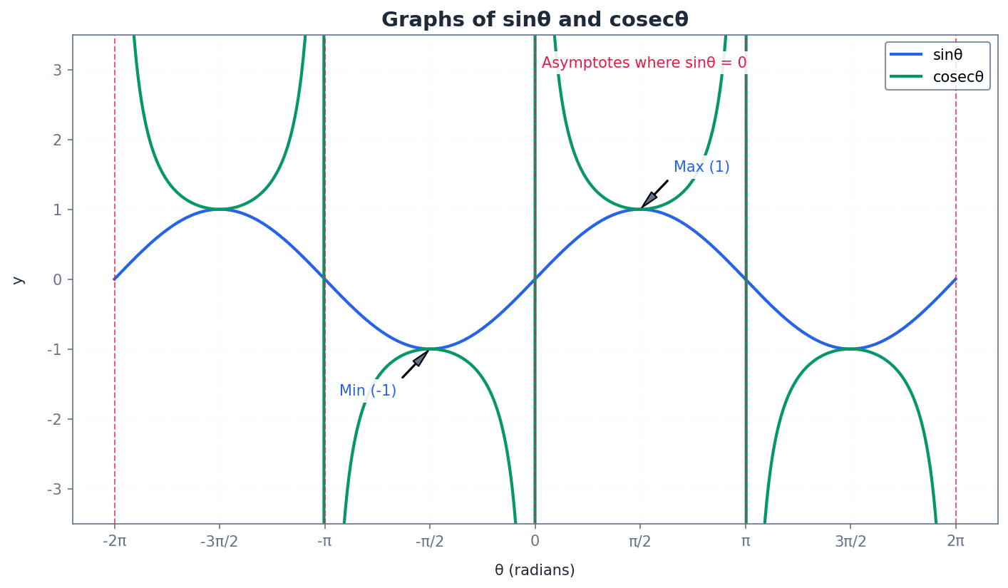
When sketching cosecθ, ensure vertical asymptotes are clearly drawn at θ = 0°, 180°, 360° and that the curve 'touches' the peaks/troughs of the sine curve.
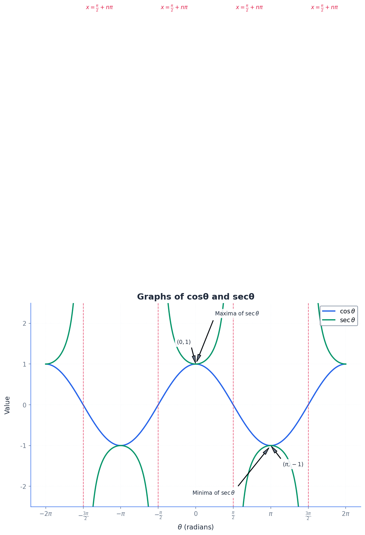
Remember that secθ is undefined when cosθ = 0, which occurs at θ = 90°, 270°. These points must be marked as asymptotes on its graph.
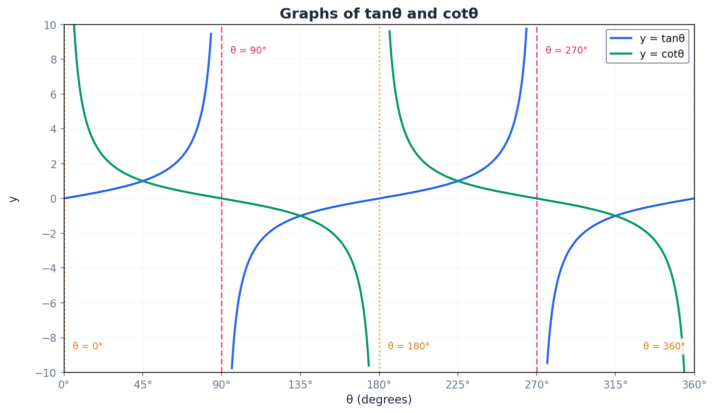
Be careful with the domain for cotθ; it is undefined when sinθ = 0, which means θ = 0°, 180°, 360°.
Trigonometric identities are fundamental for simplifying expressions and solving complex trigonometric equations. Beyond the basic reciprocal definitions, key identities include the Pythagorean identities involving cotangent and cosecant, and tangent and secant. These are derived from the primary Pythagorean identity sin²θ + cos²θ = 1 by dividing by sin²θ or cos²θ respectively.
Pythagorean identity (with cotangent and cosecant)
Derived from sin²θ + cos²θ = 1 by dividing by sin²θ
Pythagorean identity (with tangent and secant)
Derived from sin²θ + cos²θ = 1 by dividing by cos²θ
Compound angle formulae allow us to expand trigonometric functions of sums or differences of angles, such as sin(A ± B), cos(A ± B), and tan(A ± B). These are essential for exact evaluation of expressions involving non-standard angles and for simplifying more complex trigonometric equations. For example, sin 105° can be evaluated exactly by expressing it as sin(60° + 45°).
Sine compound angle formula (addition)
Used to expand the sine of a sum of two angles
Sine compound angle formula (subtraction)
Used to expand the sine of a difference of two angles
Cosine compound angle formula (addition)
Used to expand the cosine of a sum of two angles
Cosine compound angle formula (subtraction)
Used to expand the cosine of a difference of two angles
Tangent compound angle formula (addition)
Undefined if 1 - tanA tanB = 0
Tangent compound angle formula (subtraction)
Undefined if 1 + tanA tanB = 0
Errors in algebraic manipulation when expanding compound angle formulae are common, leading to incorrect identities or solutions. Pay close attention to signs and terms.
Double angle formulae are special cases of compound angle formulae, derived by setting A = B. They relate trigonometric functions of 2A to functions of A. There are three forms for cos 2A, offering flexibility in solving equations by allowing conversion to expressions solely in terms of sin A or cos A. These formulae are vital for simplifying expressions and solving equations involving angles that are multiples of each other.
Sine double angle formula
Derived from sin(A+B) by setting B=A
Cosine double angle formula (primary form)
Derived from cos(A+B) by setting B=A
Cosine double angle formula (in terms of cosine)
Derived from cos 2A = cos²A - sin²A using sin²A = 1 - cos²A
Cosine double angle formula (in terms of sine)
Derived from cos 2A = cos²A - sin²A using cos²A = 1 - sin²A
Tangent double angle formula
Derived from tan(A+B) by setting B=A; undefined if 1 - tan²A = 0
Not choosing the most suitable form of the double angle formula for cos 2A when solving equations can complicate the solution process. Select the form that simplifies the equation most effectively, often by converting to a single trigonometric function.
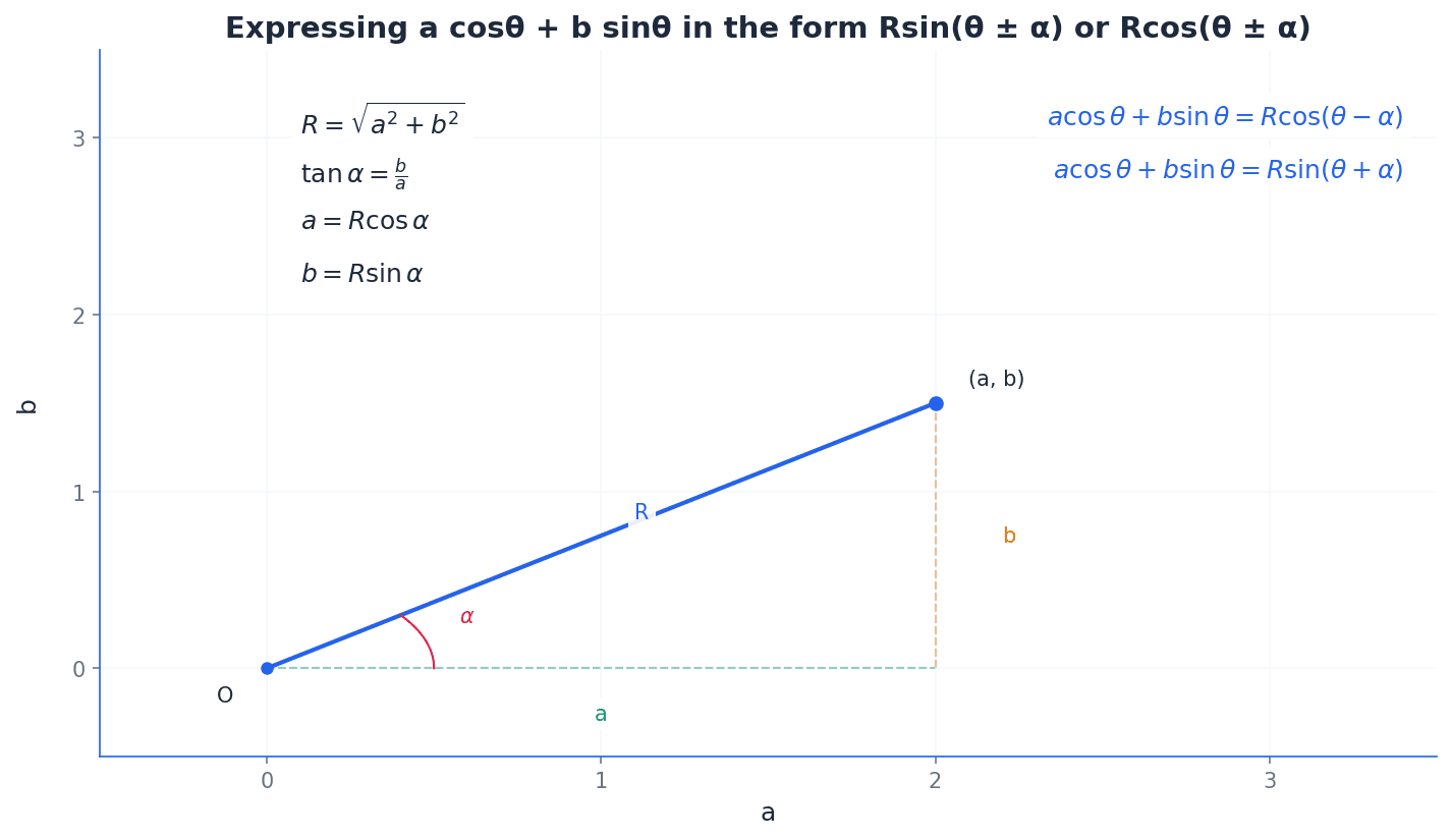
The R-form is a powerful technique for expressing a sum of sine and cosine functions, a cosθ + b sinθ, as a single sinusoidal function, such as Rsin(θ ± α) or Rcos(θ ± α). This transformation is crucial for finding the maximum and minimum values of such expressions, as the amplitude R directly corresponds to these values. It also simplifies solving equations involving these sums by reducing them to a single trigonometric equation.
R-form (Rsin(θ+α))
Where R = √(a² + b²) and tanα = b/a
R-form (Rsin(θ-α))
Where R = √(a² + b²) and tanα = b/a
R-form (Rcos(θ+α))
Where R = √(a² + b²) and tanα = b/a
R-form (Rcos(θ-α))
Where R = √(a² + b²) and tanα = b/a
Mistakes in calculating the phase angle α in R-form expressions are common, particularly with determining the correct quadrant of α or the ratio used for tan α. Always ensure α is acute (0° < α < 90°) unless otherwise specified.
When asked for the maximum or minimum value of an expression like a cosθ + b sinθ, remember it corresponds to R and -R respectively, where R is the amplitude.
Students often forget to consider all possible solutions within the given domain when solving trigonometric equations, especially after using identities. Always check for additional solutions by adding or subtracting the period of the function.
When solving equations, always state the general solution first before finding specific solutions within the given range.
For 'exact evaluation' questions, use identities and special angles (e.g., π/6, π/4, π/3) without a calculator.
When using R-form, clearly show the working for finding R and α, including the right-angled triangle or tan α calculation.
Practice sketching graphs of all six trigonometric functions, paying attention to asymptotes, intercepts, and periodicity.
When simplifying expressions, look for opportunities to apply Pythagorean, compound, or double angle identities to reduce complexity.
Exam Technique
Finding exact values of reciprocal functions
Solving trigonometric equations using identities
| Mistake | Fix |
|---|---|
| Confusing reciprocal functions (e.g., cosecθ = 1/cosθ). | Memorise the definitions: cosecθ = 1/sinθ, secθ = 1/cosθ, cotθ = 1/tanθ. |
| Incorrectly applying signs of trigonometric ratios in different quadrants. | Use the 'CAST' rule or sketch the unit circle to determine the correct sign for each quadrant. |
| Forgetting to consider all possible solutions within the given domain. | After finding the principal value, add/subtract the period (180° for tan, 360° for sin/cos) to find all solutions in the range. |
This chapter expands differentiation to include products, quotients, and composite functions involving exponential, logarithmic, and trigonometric expressions. It also introduces implicit and parametric differentiation, essential for finding derivatives of functions not explicitly defined as y=f(x) or where x and y depend on a third variable.
explicit functions — Functions where y is given explicitly in terms of x, typically in the form y = f(x).
These are the standard functions encountered in differentiation where one variable is isolated on one side of the equation. Most differentiation rules are initially introduced for explicit functions, much like a recipe where all ingredients are clearly listed and measured for one specific dish, clearly stating y's value based on x.
implicit function — A function given as an equation connecting x and y, where y is not the subject.
Implicit functions define a relationship between x and y without explicitly solving for y. Differentiating these requires the chain rule to handle terms involving y with respect to x. Imagine a tangled knot of string where you can see both ends (x and y) but can't easily pull one end free without affecting the other; an implicit function is like that knot.
parameter — A third variable, often t, used to define x and y as functions of that variable.
In parametric equations, both x and y are expressed in terms of a common independent variable, the parameter. This allows for describing curves that might not be functions in the traditional y=f(x) sense. Think of a movie director (the parameter) who tells two actors (x and y) what to do at each moment; the actors' actions (x and y values) are both dependent on the director's instructions (the parameter's value).
parametric equations — Two equations that define x and y as functions of a third variable, called a parameter.
These equations provide a way to describe a curve by specifying the coordinates (x, y) as functions of a single independent variable (the parameter). This is particularly useful for describing motion or complex shapes. For example, if you're tracking a boat's position, you might describe its longitude (x) and latitude (y) at different times (t); the equations for longitude(t) and latitude(t) are the parametric equations.
Product Rule
Used to differentiate the product of two functions, u and v, where both are functions of x.
Quotient Rule
Used to differentiate the quotient of two functions, u (numerator) and v (denominator), where both are functions of x.
Clearly identify u and v for product and quotient rules before differentiating to avoid errors. Pay close attention to the signs and order of terms in the quotient rule formula.
When a function is formed by the product or quotient of two simpler functions, the product rule or quotient rule must be applied. These rules extend basic differentiation to more complex explicit functions, allowing for the calculation of derivatives for expressions like (x^2 - 1)(4x + 5) or (x - 1) / (2x + 5).
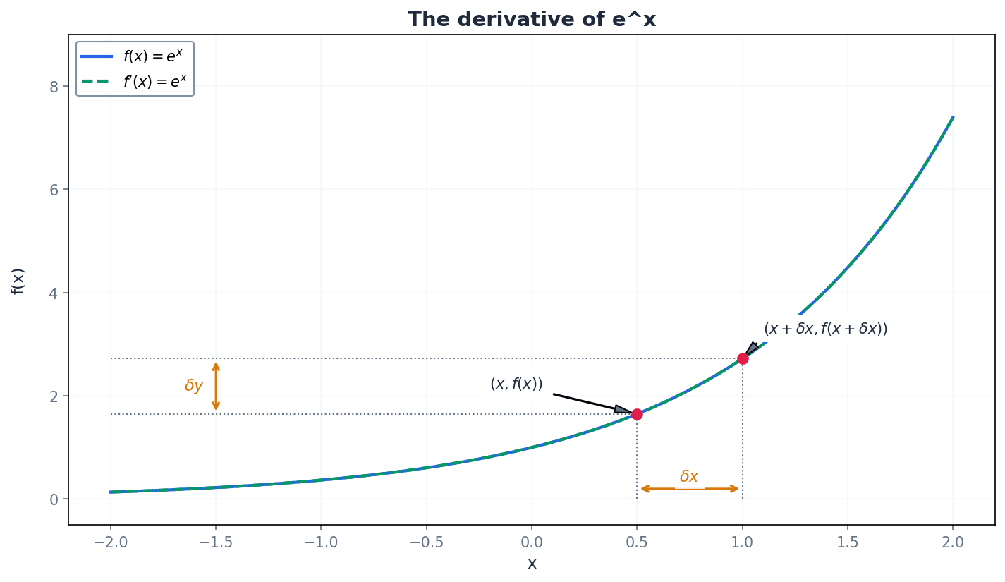
Derivative of e^x
The derivative of the natural exponential function is itself.
Derivative of e^(ax+b)
This is the chain rule applied to the exponential function, where 'a' and 'b' are constants.
Derivative of e^f(x)
This is the general chain rule for exponential functions, where f(x) is any function of x and f'(x) is its derivative.
The natural exponential function, e^x, has the unique property that its derivative is itself. For composite exponential functions like e^(ax+b) or e^f(x), the chain rule is applied, multiplying by the derivative of the exponent. This allows for differentiating expressions such as e^(3x+2) or (x^2 - 7)e^x.
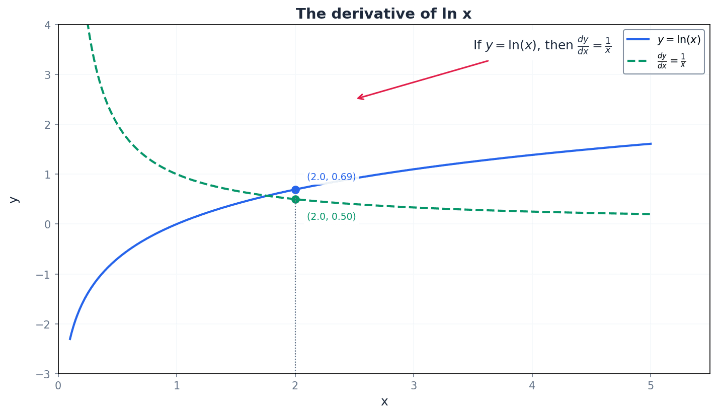
Derivative of ln x
This formula is valid for x > 0.
Derivative of ln(ax+b)
This is the chain rule applied to the natural logarithmic function, where 'a' and 'b' are constants.
Derivative of ln(f(x))
This is the general chain rule for natural logarithmic functions, where f(x) is any function of x and f'(x) is its derivative.
The derivative of ln x is 1/x, provided x > 0. For composite logarithmic functions, the chain rule is used, resulting in the derivative of the inner function divided by the inner function itself. Logarithm rules can sometimes simplify expressions before differentiation, as seen with ln((5x - 2)^3).
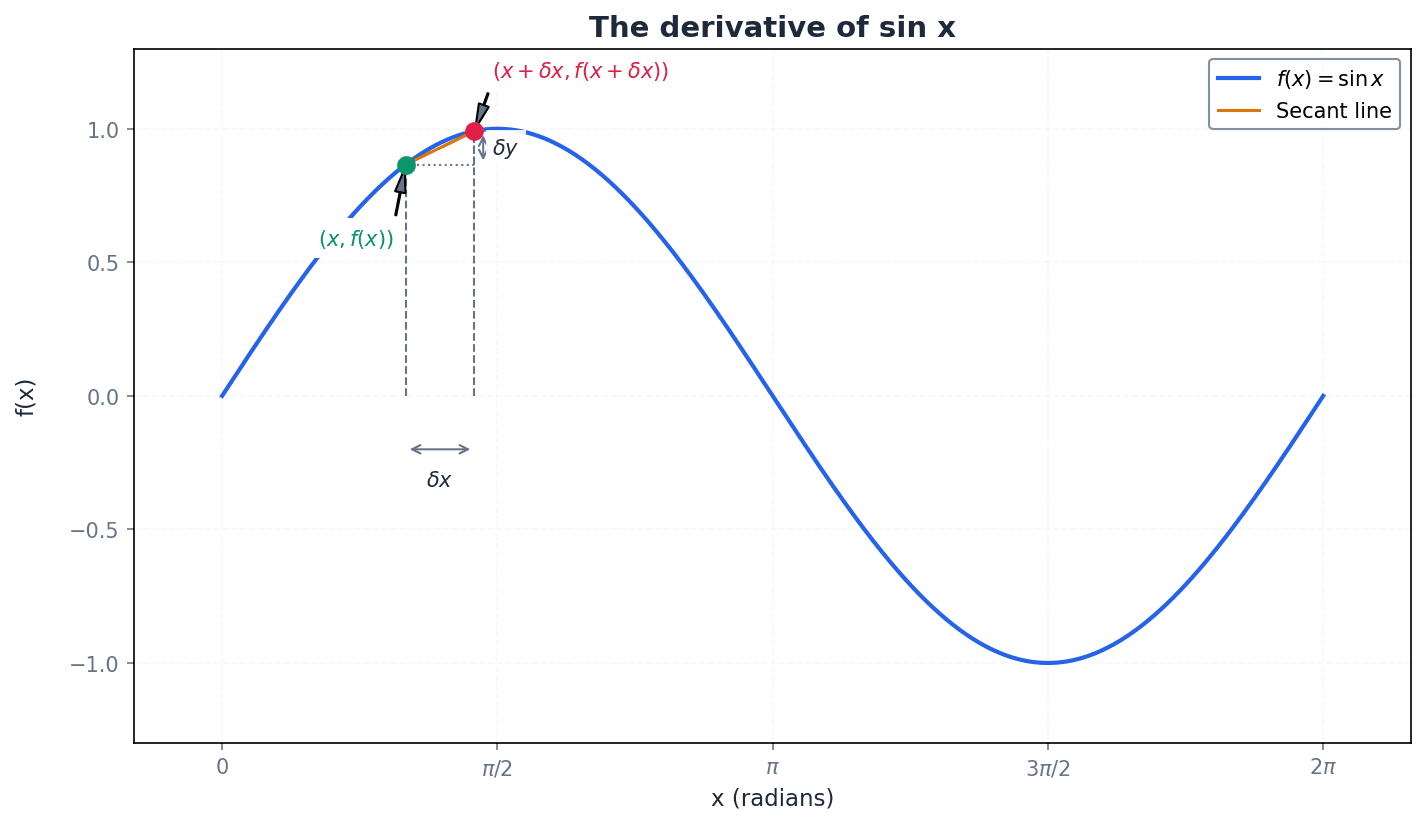
Derivative of sin x
Angles must be in radians for this formula to be valid.
Derivative of cos x
Angles must be in radians for this formula to be valid.
Derivative of tan x
Angles must be in radians for this formula to be valid.
Derivative of sin(ax+b)
This is the chain rule applied to the sine function; angles must be in radians.
Derivative of cos(ax+b)
This is the chain rule applied to the cosine function; angles must be in radians.
Derivative of tan(ax+b)
This is the chain rule applied to the tangent function; angles must be in radians.
The derivatives of sin x, cos x, and tan x are cos x, -sin x, and sec^2 x respectively, provided angles are measured in radians. For composite trigonometric functions like sin(ax+b), the chain rule is applied, multiplying by the derivative of the inner function (ax+b).
Students sometimes forget that trigonometric derivatives (sin, cos, tan) require angles to be in radians. Always ensure your calculator is in radian mode when working with these derivatives.
Implicit differentiation is used for functions where y is not explicitly given in terms of x, but rather an equation connects x and y. This method involves differentiating every term in the equation with respect to x, applying the chain rule to any term involving y by multiplying its derivative by dy/dx.
Students often forget to apply the chain rule when differentiating terms involving y in implicit differentiation, treating y as a constant or differentiating it with respect to y instead of x. Remember to multiply by dy/dx for each term involving y.
When performing implicit differentiation, differentiate each term carefully and collect all dy/dx terms to one side of the equation before solving for dy/dx.
Students might try to rearrange implicit functions into explicit form before differentiating, which is often difficult or impossible and unnecessary. Implicit differentiation allows direct differentiation without rearrangement.
Parametric Differentiation (dy/dx)
Used to find the gradient of a curve defined by parametric equations, where x and y are functions of a parameter t.
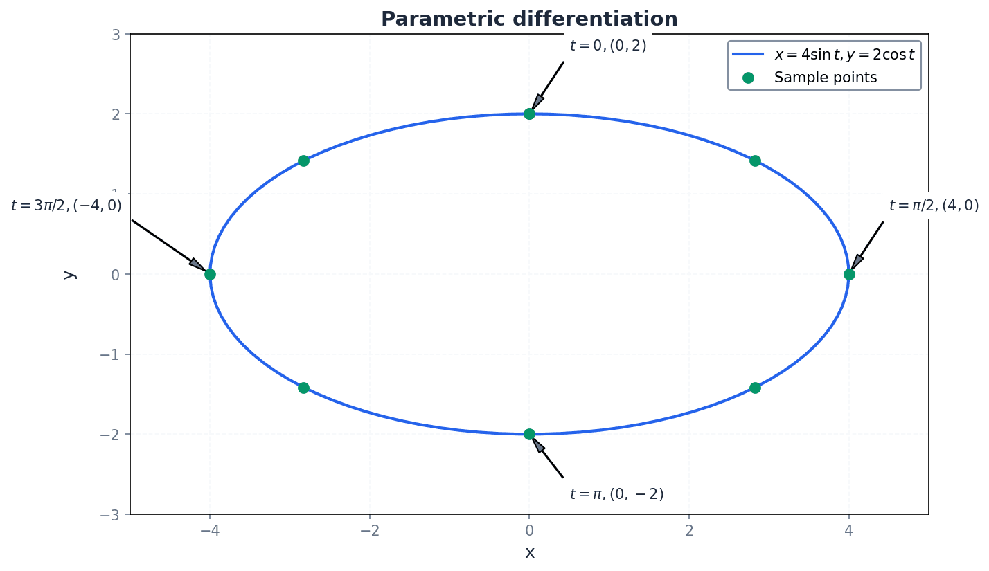
Parametric differentiation is employed when both x and y are defined as functions of a third variable, known as a parameter (often t). To find dy/dx, we first find dy/dt and dx/dt, then use the chain rule: dy/dx = (dy/dt) / (dx/dt). This method is crucial for describing curves that cannot be easily represented in the form y=f(x).
When differentiating parametrically, ensure you find dx/dt and dy/dt first, then use the chain rule (dy/dx = (dy/dt) / (dx/dt)) to find the gradient in terms of the parameter.
When finding stationary points for parametric equations, students might incorrectly set dy/dt = 0 instead of dy/dx = 0. Remember that tangents parallel to the x-axis occur when dy/dx = 0, while tangents parallel to the y-axis occur when dx/dt = 0.
Always check if the question asks for the derivative in terms of x, y, or t, and simplify your final answer accordingly.
For all differentiation problems, carefully identify the type of function (product, quotient, composite, implicit, parametric) to select the correct differentiation method. Practice applying the chain rule consistently across all function types.
Exam Technique
Differentiating products of functions
Differentiating quotients of functions
| Mistake | Fix |
|---|---|
| Forgetting the chain rule in implicit differentiation for terms involving y. | Always remember that when differentiating a term like y^n with respect to x, it becomes ny^(n-1) * dy/dx. Treat y as a function of x. |
| Confusing the product rule and quotient rule formulas. | Memorise both formulas precisely. A common mnemonic for the quotient rule is 'low d high minus high d low, over low squared' (v(du/dx) - u(dv/dx)) / v^2. |
| Using degrees instead of radians for trigonometric derivatives. | Always ensure your calculator is in radian mode when differentiating or evaluating trigonometric functions in calculus problems. The formulas d/dx(sin x) = cos x, etc., are only valid for radians. |
This chapter extends integration to include exponential, logarithmic, and trigonometric functions, building on the concept of reverse differentiation. It also covers the use of trigonometric identities to simplify integrands and introduces the trapezium rule as a numerical method for estimating definite integrals.
definite integral — An integral evaluated between two specified limits, representing the net signed area under a curve over a given interval.
Unlike indefinite integrals which result in a function plus a constant of integration, a definite integral yields a numerical value. This value can represent quantities like area, volume, or displacement, and is calculated by evaluating the antiderivative at the upper and lower limits and subtracting the results. If an indefinite integral is like finding a general recipe for a cake, a definite integral is like baking a specific cake for a party, where the limits define the exact ingredients and baking time to get a particular outcome.
trapezium rule — A numerical method used to estimate the value of a definite integral by splitting the area under the curve into equal width strips and summing the areas of the resulting trapeziums.
This rule provides an approximate answer for definite integrals when algebraic integration is not possible or specifically requested. The accuracy of the estimate increases with the number of strips used. It involves calculating the area of each strip using the formula for a trapezium and summing them. Imagine trying to measure the area of a pond with an irregular shape. Instead of trying to find an exact formula, you could divide the pond into many narrow rectangular or trapezoidal sections, measure each section, and add them up to get a good estimate of the total area.
ordinates — The lengths of the vertical edges of the strips used in the trapezium rule, corresponding to the y-values of the function at specific x-intervals.
In the context of the trapezium rule, ordinates are the y-coordinates of the points on the curve at the boundaries of each strip. These values are crucial for calculating the area of each trapezium, as they represent the parallel sides of the trapeziums. Think of a fence made of vertical posts of varying heights. The ordinates are the heights of these individual posts, which define the shape of the fence line.
Integration of exponential function
Applies when integrating exponential functions of the form e^(ax+b).
Integration of 1/(ax+b)
Valid for ax+b \neq 0. The modulus sign ensures the logarithm is defined for all valid values of x.
Students may incorrectly apply the integration rules for 1/(ax+b) without the modulus sign, leading to undefined logarithms for negative arguments. Remember to include the modulus sign for ln|ax+b| to ensure the logarithm is defined.
Integration of sin(ax+b)
Applies when integrating sine functions. x must be measured in radians.
Integration of cos(ax+b)
Applies when integrating cosine functions. x must be measured in radians.
Integration of sec^2(ax+b)
Applies when integrating secant squared functions. x must be measured in radians.
Students often confuse the differentiation and integration rules for trigonometric functions, especially the signs and coefficients. Don't confuse the signs and coefficients when integrating trigonometric functions with their differentiation rules.
Integration is fundamentally the reverse process of differentiation. This chapter extends this idea to a broader range of functions, including exponential, logarithmic, and trigonometric forms. Understanding the corresponding differentiation rules is key to correctly applying these new integration techniques.
The integration of exponential functions of the form follows a direct rule, yielding . Similarly, functions of the form integrate to . It is crucial to remember the modulus sign for the logarithmic term to ensure the function is defined for all valid values of x.
The integration of basic trigonometric functions like , , and also follows specific rules, involving a reciprocal of the coefficient 'a' and a change in sign for sine functions. For more complex trigonometric integrands, such as or , trigonometric identities are often necessary to rewrite the expression into a form that can be integrated using the standard rules. This simplification is a critical step before proceeding with integration.
Always check if trigonometric relationships can simplify the integrand before attempting integration.
Students often forget to add the constant of integration 'c' for indefinite integrals. Don't forget to add the constant of integration 'c' for indefinite integrals.
Definite integrals are evaluated between two specified limits, resulting in a numerical value rather than a function with a constant of integration. This value often represents the net signed area under a curve over a given interval. When evaluating definite integrals, substitute the upper limit first, then the lower limit, and subtract the results, paying close attention to signs.
Always substitute the upper limit first, then the lower limit, and subtract the results. Pay close attention to signs, especially when dealing with trigonometric functions or negative values.
Trapezium Rule
Used to approximate definite integrals. h = (b-a)/n. The number of ordinates is n+1.
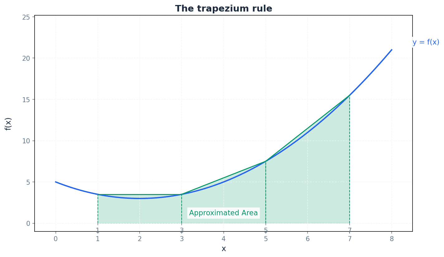
When algebraic integration is not feasible or specifically requested, the trapezium rule offers a numerical method to estimate definite integrals. It works by dividing the area under the curve into equal-width strips and approximating each strip as a trapezium. The sum of these trapezium areas provides an estimate of the total definite integral. The accuracy of this estimate improves with an increased number of strips.
Students often think the trapezium rule gives the exact answer, but actually it provides an estimate, which can be an under-estimate or an over-estimate depending on the curve's concavity. Don't use the trapezium rule if an exact algebraic method is available and not specifically asked for.
Students often think the number of ordinates is the same as the number of strips, but actually the number of ordinates is one more than the number of strips. Don't incorrectly count the number of ordinates versus the number of strips in the trapezium rule (n strips = n+1 ordinates).
When asked to 'state, with a reason, whether the trapezium rule gives an under-estimate or an over-estimate', you must refer to the shape of the curve (concave or convex) relative to the top edges of the trapeziums.
Students often struggle to correctly identify whether the trapezium rule gives an under-estimate or an over-estimate, failing to link it to the concavity/convexity of the curve. Don't struggle to identify if the trapezium rule gives an under-estimate or over-estimate; link it to the curve's concavity.
For trapezium rule questions, clearly show your calculation of 'h' and list your ordinates (y-values) to avoid calculation errors.
If a question doesn't specify a method, consider if an exact algebraic integration is possible before resorting to numerical methods like the trapezium rule.
Exam Technique
Integrate exponential functions
Integrate functions of the form 1/(ax+b)
| Mistake | Fix |
|---|---|
| Forgetting the constant of integration 'c' for indefinite integrals. | Always add '+ c' at the end of any indefinite integral. |
| Omitting the modulus sign in $\ln|ax+b|$, leading to undefined logarithms. | Always use $|ax+b|$ to ensure the logarithm is defined for all valid x values. |
| Confusing the signs or coefficients when integrating trigonometric functions (e.g., $\int \sin(ax+b) dx$ vs. $\frac{d}{dx} \cos(ax+b)$). | Practice differentiation and integration rules side-by-side to solidify the correct signs and coefficients. Remember integration is the reverse process. |
This chapter introduces numerical methods for solving equations that cannot be solved algebraically, focusing on locating approximate roots and refining them using iterative processes. It covers graphical analysis, the change of sign method, and understanding how iterative formulae converge to a root.
Numerical methods — Numerical methods are ways of calculating approximate solutions to equations.
These methods are used when direct algebraic solutions are not possible or are too complex. They are powerful problem-solving tools widely used in various applications like engineering and finance. Imagine trying to find the exact height of a mountain; you use surveying tools to get closer and closer approximations, just like numerical methods find approximate solutions.
Students often think numerical methods give exact answers, but actually they provide approximations that can be made arbitrarily accurate. Also, don't assume all equations can be solved algebraically; many require numerical approximations.
Root — The values of x that make both sides of an equation equal are called the roots of the equation.
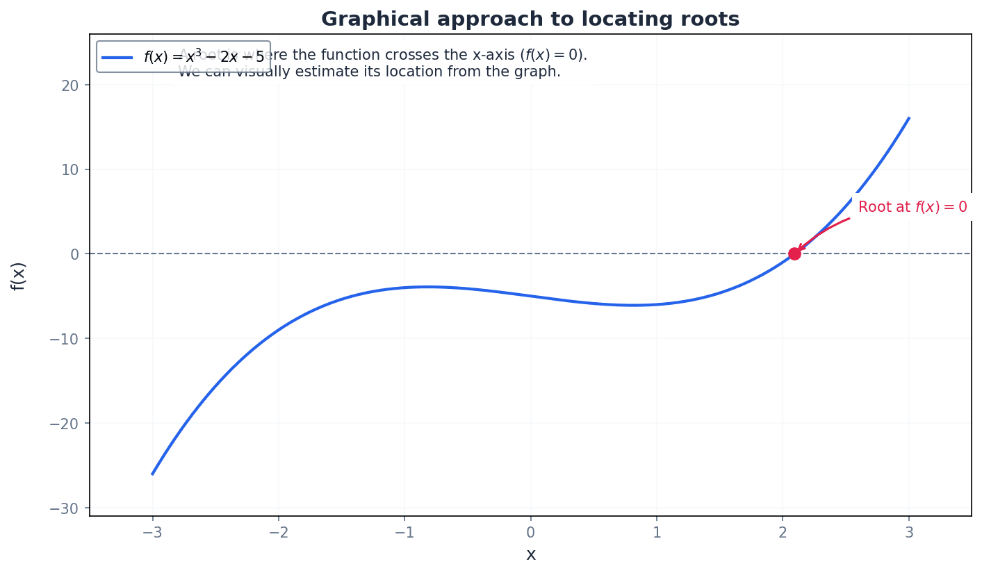
Graphically, the roots of f(x) = 0 are the x-intercepts on the graph of y = f(x). In the context of iterative methods, we aim to find these roots to a prescribed degree of accuracy. Think of a root as the 'target' value you're trying to hit; it's the specific number that makes the equation true, like the bullseye on a dartboard.
Students often think 'root' only refers to square roots, but actually it's a general term for any solution to an equation. Also, students may confuse the graphical intersection of y=f(x) and y=g(x) with the roots of f(x)=0; the roots are the x-intercepts of y=f(x).
Before applying iterative methods, it's crucial to locate an approximate root. This can be done using graphical considerations or the change of sign method. Graphical analysis involves sketching relevant functions to identify intersection points, while the change of sign method uses function evaluations to pinpoint intervals containing a root.
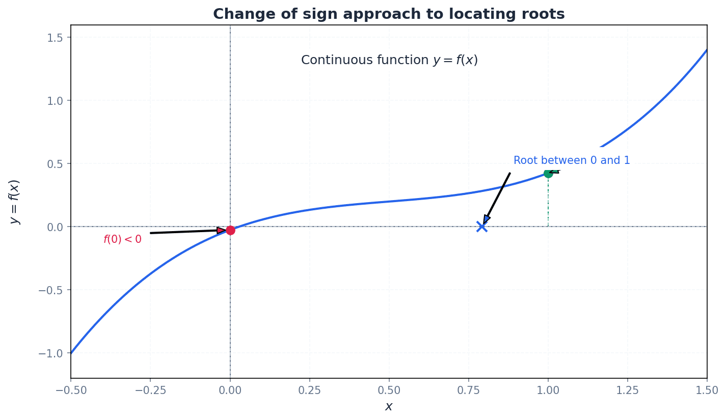
When asked to 'show that a root lies between two values', this typically requires a change of sign calculation and a concluding statement. Remember that a change of sign only indicates a root if the function is continuous over the interval.
Iterative formula — A relationship such as x_n+1 = F(x_n) where x_n+1 = F(x_n) is the basis for an iterative formula.
This formula defines a sequence of approximations where each term is derived from the previous one, leading towards the root of an equation. The choice of F(x) and the starting value x_1 are crucial for convergence. It's like a recipe for finding a treasure: you follow the instructions (the formula) using your current location (x_n) to find a new, better location (x_n+1) until you reach the treasure (the root).
Iterative formula
Used to generate a sequence of values that converge to a root of an equation f(x)=0, where f(x)=0 has been rearranged into the form x=F(x).
Students often think any rearrangement of f(x)=0 into x=F(x) will work, but actually some rearrangements lead to divergent sequences. Also, students may assume any rearrangement of f(x)=0 into x=F(x) will lead to a convergent iterative formula, but some rearrangements cause divergence.
Always state the iterative formula clearly before applying it. When asked to derive a formula, ensure it is a valid rearrangement of the original equation. Be precise with notation: use x_n and x_n+1 correctly to represent successive approximations in iterative formulae.
Iteration — Each test in an iterative process is called an iteration.
An iteration involves substituting a current approximation into an iterative formula to generate a new, hopefully more accurate, approximation of the root. This process is repeated until the desired accuracy is achieved. It's like refining a sculpture: each time you chip away a bit of stone, you're making an 'iteration' to get closer to the final shape.
Students often think that a single iteration is enough, but actually multiple iterations are usually required to achieve the desired level of accuracy. Also, students often round intermediate iteration values too early, leading to inaccuracies in the final answer.
When performing iterations, show the result of each step to a suitable number of decimal places (usually more than the final required accuracy) to avoid premature rounding errors.
Converging — When the point of intersection is at x = α and your iterations are values that are getting closer and closer to α, you are converging to α.
Convergence means that the sequence of approximations generated by the iterative formula approaches a specific limit, which is the root of the equation. This is visually represented by cobweb or staircase patterns. Imagine a spiral staircase leading down to a specific point; each step you take gets you closer to that point, just as each iteration gets closer to the root.
Students often think that if the values are changing, they are converging, but actually the values must be getting progressively closer to a single limit.
The graphical representation of an iterative process, plotting y=x and y=F(x), reveals distinct convergence patterns. These patterns, known as cobweb and staircase, illustrate how the sequence of approximations approaches the root. Understanding these patterns helps visualise the behaviour of the iterative formula.
Cobweb pattern — The spiral pattern of convergence seen when plotting y=x and y=F(x) for an iterative process is often called the cobweb pattern.
This pattern occurs when the gradient of F(x) at the root is between -1 and 0, or between 0 and 1, and the iterations 'spiral' inwards towards the intersection point. It's like a spider spinning a web, where the lines of the iteration move back and forth, getting tighter and tighter around the center (the root).
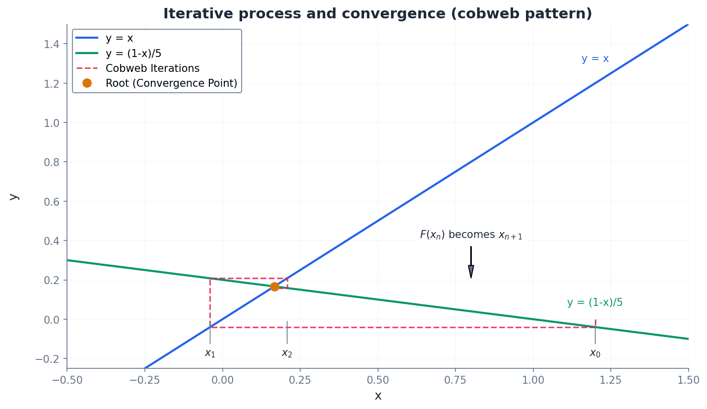
Students often think the cobweb pattern always means convergence, but actually it only converges if the gradient of F(x) at the root is within the range (-1, 1).
Staircase pattern — The type of convergence shown in a graph where iterations move in a 'staircase' fashion towards the root is often called a staircase pattern.
This pattern typically occurs when the gradient of F(x) at the root is positive and between 0 and 1, causing the iterations to approach the root monotonically. Imagine walking up or down a set of stairs towards a specific landing; each step brings you closer to that landing, just as each iteration brings you closer to the root.
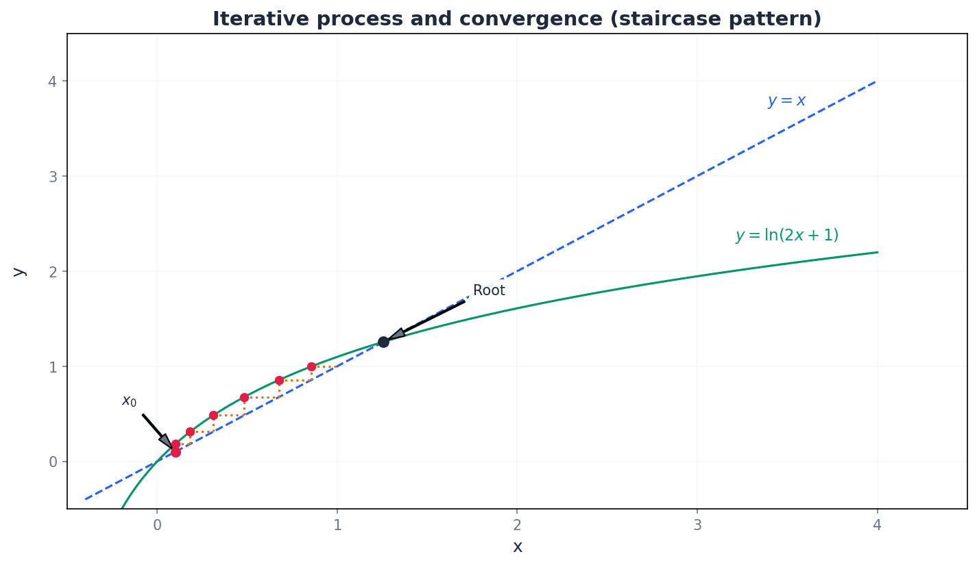
Students often think the staircase pattern is always faster than the cobweb, but actually the speed of convergence depends on the magnitude of the gradient of F(x) at the root.
Once an iterative process has converged to an approximate root, its accuracy to a prescribed degree (e.g., decimal places or significant figures) must be verified. This is typically done using a change of sign test on the original function f(x) at the boundaries of the required interval.
Students might not use the change of sign test correctly to prove the accuracy of a root to a prescribed number of decimal places or significant figures.
To prove convergence to a certain decimal place, use the change of sign test on the original function f(x) with values slightly above and below the rounded root. For 'prescribed degree of accuracy', use the change of sign test on the original function f(x) at the upper and lower bounds of the required interval.
Clearly show your iterative steps, including the formula and at least the first few iterations, before stating the final root. If an iterative formula is given, use it directly; if you need to derive one, ensure your rearrangement x=F(x) is valid and likely to converge.
Exam Technique
Locating a root using graphical considerations
Locating a root using the change of sign method
| Mistake | Fix |
|---|---|
| Rounding intermediate iteration values too early. | Maintain full calculator accuracy for intermediate steps. Only round the final answer to the required degree of accuracy after the change of sign test. |
| Assuming any rearrangement of f(x)=0 into x=F(x) will converge. | Be aware that some rearrangements lead to divergent sequences. If an iteration diverges, try a different rearrangement if possible. The gradient of F(x) at the root must be between -1 and 1 for convergence. |
| Incorrectly applying the change of sign test for accuracy. | To prove a root is accurate to 'd' decimal places, test f(x) at x - 0.5 * 10^(-d) and x + 0.5 * 10^(-d). For 's' significant figures, test at the appropriate bounds. Always use the original function f(x) for this test. |
This chapter introduces advanced algebraic techniques for Pure Mathematics 3, focusing on decomposing rational functions into partial fractions and applying the general binomial theorem for non-positive integer powers. Students will learn to handle various denominator forms and combine these skills to expand complex rational expressions into series.
partial fractions — Partial fractions is the reverse process of adding or subtracting algebraic fractions, where a single algebraic fraction is split into two or more simpler fractions.
This decomposition simplifies complex rational expressions, making them easier to integrate, differentiate, or expand using binomial series. Imagine you have a complex machine that's hard to fix. Splitting it into its simpler components (partial fractions) makes it easier to understand and work with each part individually. Different forms of partial fractions are used depending on the nature of the denominator's factors.
algebraic improper fraction — An algebraic fraction P(x)/Q(x) is an algebraic improper fraction if the degree of P(x) is greater than or equal to the degree of Q(x).
This means the numerator polynomial has a degree equal to or higher than the denominator polynomial. Similar to how 11/5 is an improper numerical fraction that can be written as 2 + 1/5, an algebraic improper fraction like (x^3 + 2x)/(x - 1) can be written as a polynomial plus a proper algebraic fraction. Such fractions must be converted into a sum of a polynomial and a proper fraction before applying partial fraction decomposition.
telescoping series — A telescoping series is a series whose partial sums only have a fixed number of terms after cancellation.
This cancellation occurs because intermediate terms in the sum cancel each other out, leaving only the first and last few terms. Imagine a collapsible telescope: when you extend it, many segments are visible, but when you collapse it, only the end pieces remain. This property makes it possible to find the sum to infinity of such series.
Partial fraction form for distinct linear factors
Used when the denominator has two distinct linear factors. This form can be extended for more linear factors.
Partial fraction form for repeated linear factors
Used when the denominator has a repeated linear factor. For (ax+b)^3, an additional term C/(ax+b)^3 would be included.
Partial fraction form for irreducible quadratic factors
Used when the denominator has a linear factor and an irreducible quadratic factor of the form cx^2+d.
The process of partial fraction decomposition involves splitting a complex rational expression into simpler fractions. The specific form of the partial fractions depends on the nature of the denominator's factors. There are distinct forms for distinct linear factors, repeated linear factors, and irreducible quadratic factors. This technique is crucial for simplifying expressions before further operations like integration or binomial expansion.
Students often think that improper algebraic fractions can be directly decomposed into partial fractions, but actually they must first be expressed as a sum of a polynomial and a proper fraction.
Ensure you choose the correct form for the partial fraction decomposition based on whether the denominator has distinct linear factors, repeated linear factors, or irreducible quadratic factors.
Students often think that a quadratic factor in the denominator can always be factorised, but actually some quadratic factors (like x^2+1) are irreducible and require a Bx+C form in the numerator of the partial fraction.
Students often think that for repeated linear factors, only one term is needed (e.g., A/(ax+b)^2), but actually terms for all powers up to the repeated factor are needed (e.g., A/(ax+b) + B/(ax+b)^2).
General binomial theorem for rational n
This series is infinite and is only valid for |x| < 1. Here, 'n' represents any rational number.
Binomial expansion of (a+x)^n
This form is used when the first term in the bracket is not 1. The expansion is valid for |x/a| < 1, which simplifies to |x| < |a|.
The general binomial theorem extends the concept of binomial expansion to cases where the power 'n' is a rational number, including negative integers or fractions. Unlike expansions for positive integer powers, these series are infinite. It is crucial to remember that these expansions are only valid for a specific range of x values, typically |x| < 1 for the (1+x)^n form, or |x| < |a| for (a+x)^n.
Students often think that the binomial expansion for non-positive integer powers is always valid, but actually it is only valid for |x| < 1 (or |x/a| < 1 for (a+x)^n).
Complex rational expressions can often be expanded into series by first decomposing them into partial fractions. Each simpler partial fraction can then be rewritten into the (1+kx)^n form, allowing the application of the binomial theorem. This combined approach enables the expansion of expressions that would otherwise be difficult to handle directly.
Students often think that when combining partial fractions and binomial expansions, the range of validity is the union of individual ranges, but actually it is the intersection of all valid ranges.
When asked to express an improper algebraic fraction in partial fractions, always perform polynomial long division first to obtain a polynomial and a proper fraction, then decompose the proper fraction.
To identify a telescoping series, look for terms that can be expressed as a difference, such that when summed, intermediate terms cancel out. Partial fractions are often used to achieve this difference form.
Clearly state the range of validity for any binomial expansion, as this is often a separate mark.
When finding constants for partial fractions, use a combination of substitution (for linear factors) and equating coefficients (for quadratic or repeated factors) for efficiency.
When applying binomial expansion to partial fractions, ensure each term is in the (1+kx)^n form before expanding.
Exam Technique
Decompose a proper rational function into partial fractions (distinct linear factors)
Decompose a proper rational function into partial fractions (repeated linear factors)
| Mistake | Fix |
|---|---|
| Forgetting to perform polynomial long division for improper algebraic fractions. | Always check the degree of the numerator and denominator. If degree(P(x)) >= degree(Q(x)), perform long division first. |
| Incorrectly setting up partial fraction forms, especially for repeated linear factors or irreducible quadratic factors. | Memorise the correct forms: A/(ax+b) + B/(ax+b)^2 for repeated factors, and A/(ax+b) + (Bx+C)/(cx^2+d) for irreducible quadratics. |
| Not stating or incorrectly determining the range of validity for binomial expansions. | Always include the validity condition |X| < 1 (where X is the 'x' term in (1+X)^n) and simplify it for the variable x. For combined expansions, find the intersection of all ranges. |
This chapter introduces advanced integration techniques, building upon prior calculus knowledge. It covers the integration of specific function forms, such as those involving inverse tangent and logarithmic functions, and powerful methods like integration by substitution and integration by parts. Additionally, it details the integration of rational functions through partial fraction decomposition.
Indefinite integral — The general form of the antiderivative of a function, including an arbitrary constant of integration.
An indefinite integral represents the family of all functions whose derivative is the given function. The constant of integration, 'C', is crucial as it accounts for the fact that the derivative of any constant is zero, meaning there are infinitely many antiderivatives.
Definite integral — An integral evaluated between two specified limits, representing the net signed area under a curve.
Unlike indefinite integrals, which result in a function plus a constant, definite integrals yield a numerical value. When using substitution with definite integrals, it is essential to convert the original limits of integration to the new variable to ensure accuracy.
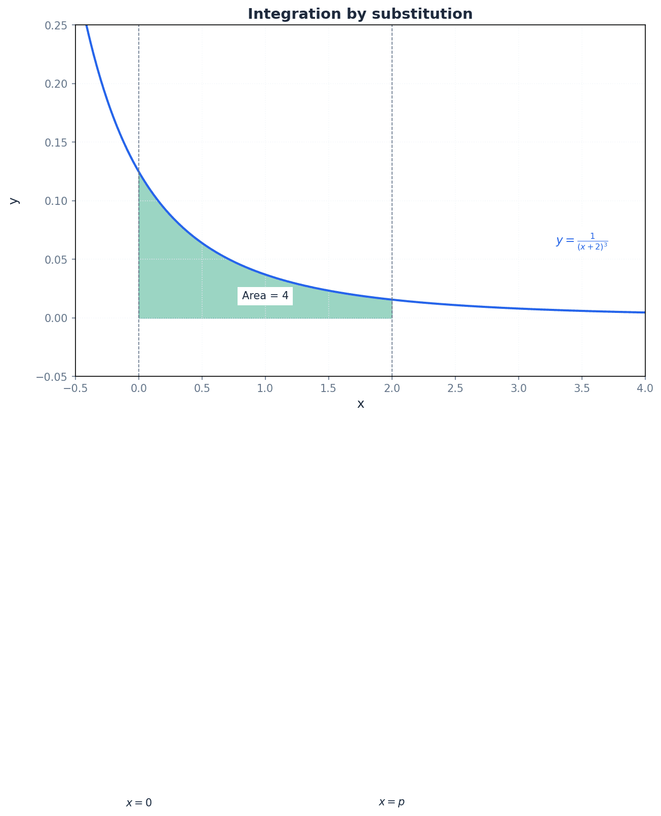
Integration by substitution — A method used to transform a difficult integral into an easier integral by applying a simple substitution.
This technique is considered the reverse process of differentiation by the chain rule. Imagine you have a complex puzzle, and you swap out a difficult piece for a simpler one that fits perfectly, making the rest of the puzzle easier to solve. The substitution is like that simpler piece, simplifying the integral.
Students often think they only need to substitute the variable when using integration by substitution, but actually they must also convert the differential (dx) and, for definite integrals, the limits of integration to the new variable.
When using substitution for definite integrals, always remember to convert the limits to the new variable. Failure to do so is a common error that leads to incorrect answers.
Integration by parts — A technique used to integrate a product of two functions by applying a specific formula derived from the product rule for differentiation.
This method is particularly useful when direct integration or substitution is not feasible for a product of functions. Think of it like 'un-doing' the product rule. It involves choosing one part of the integrand to differentiate (u) and the other to integrate (dv/dx) to simplify the overall integral.
Students often think the choice of 'u' and 'dv/dx' doesn't matter in integration by parts, but actually choosing them carefully (e.g., 'u' as a function that simplifies when differentiated) is crucial for the integral to become easier.
When applying integration by parts, carefully choose 'u' and 'dv/dx'. A good strategy is to choose 'u' as the function that becomes simpler when differentiated (e.g., ln x, polynomials) and 'dv/dx' as the function that is easily integrated.
Partial fractions — A method of decomposing a rational function into a sum of simpler fractions.
This technique is used to integrate rational functions where the denominator can be factorised. Imagine you have a complicated mixed drink, and you want to understand its components. Partial fractions is like separating that drink back into its individual ingredients, which are easier to analyse (or in this case, integrate).
Students often think partial fractions only apply to proper fractions, but actually improper fractions must first be divided (numerator by denominator) before decomposition into partial fractions.
For rational functions where the degree of the numerator is greater than or equal to the degree of the denominator, perform algebraic long division first before attempting to decompose into partial fractions.
Derivative of tan⁻¹x
Used for differentiating the inverse tangent function.
Derivative of tan⁻¹(ax)
This is an extension of the derivative of tan⁻¹x using the chain rule, where 'a' is a constant.
Derivative of tan⁻¹(f(x))
This is the general form for differentiating the inverse tangent of any function of x, f(x), using the chain rule.
The derivative of tan⁻¹x provides a direct path to integrating functions of the form 1/(a² + x²). By recognising this specific structure, we can reverse the differentiation process to find the integral. For example, to differentiate tan⁻¹(3x), we apply the chain rule, resulting in 3/(1 + (3x)²).
Integral of 1/(a² + x²)
This formula is used for integrating functions that can be expressed in the form 1/(a² + x²), where 'a' is a constant. Remember to include the constant of integration, C.
A common and powerful integration technique involves recognising when the numerator of a fraction is the derivative of its denominator. This specific form allows for direct integration to a logarithmic function. For instance, to integrate tan(3x), it can be rewritten as sin(3x)/cos(3x), where the numerator is a multiple of the derivative of the denominator.
Integral of f'(x)/f(x)
This formula is used for integrating functions where the numerator is the derivative of the denominator. It is important that f(x) > 0 for ln f(x) to exist, hence the absolute value. 'C' is the constant of integration.
Integration by substitution is a versatile method for simplifying complex integrals. It works by transforming the integral into a simpler form using a new variable. This technique is essentially the reverse of the chain rule in differentiation. When applying substitution, it is crucial to rewrite the entire integral, including the differential (dx) and, for definite integrals, the limits of integration, in terms of the new variable.
Rational functions, which are ratios of polynomials, can often be integrated by first decomposing them into partial fractions. This method breaks down a complex fraction into a sum of simpler fractions, each of which can then be integrated using standard techniques, frequently resulting in logarithmic terms. This approach is particularly effective when the denominator of the rational function can be factorised.
Integration by parts is a powerful technique specifically designed for integrating products of two functions. It is derived directly from the product rule for differentiation. The method involves strategically choosing one part of the integrand to be 'u' (which will be differentiated) and the other part to be 'dv/dx' (which will be integrated), aiming to simplify the integral after applying the formula.
Students often forget to include the constant of integration '+ C' for indefinite integrals. Its omission will result in loss of marks as it represents the entire family of antiderivatives.
Always remember to include the constant of integration '+ C' when finding indefinite integrals. Its absence is a common reason for losing marks in examinations.
Be prepared to combine multiple integration techniques within a single problem, such as substitution followed by partial fractions, as complex integrals often require a sequence of methods.
Exam Technique
Differentiating tan⁻¹(f(x))
Integrating 1/(a² + x²)
| Mistake | Fix |
|---|---|
| Forgetting to convert the differential (dx) when performing integration by substitution. | Always write dx in terms of du (e.g., if u=3x, then du/dx=3, so dx=du/3) and substitute it into the integral. |
| Forgetting to convert the limits of integration when performing definite integrals with substitution. | Before integrating, calculate the new upper and lower limits for the substituted variable 'u' using the substitution equation. Evaluate the integral directly with these new limits. |
| Choosing 'u' and 'dv/dx' incorrectly in integration by parts, leading to a more complex integral. | Prioritise 'u' as functions that simplify when differentiated (e.g., ln x, polynomials) and 'dv/dx' as functions that are easily integrated (e.g., e^x, sin x, cos x). The LIATE rule (Logarithmic, Inverse trig, Algebraic, Trigonometric, Exponential) can be a helpful guide for choosing 'u'. |
This chapter introduces vectors in two and three dimensions, covering their notation, arithmetic, and geometric interpretation. It explains how to calculate magnitudes, find unit vectors, and distinguish between displacement and position vectors. Key topics include finding the vector equation of a line, determining relationships between lines, and using the scalar product to find angles or test for perpendicularity.
displacement — A movement through a certain distance and in a given direction.
Displacement vectors, also known as translation vectors, represent the change in position from a starting point to an end point. They have both magnitude (distance moved) and direction. For example, if you walk 100m north from your house, your displacement is 100m north, regardless of the path you took to get there.
translation — A movement through a certain distance and in a given direction.
Translation is synonymous with displacement in the context of vectors, describing the shift of an object or point from one position to another without rotation or scaling. It is represented by a vector. Moving a chess piece from one square to another is a translation; the vector describes how far and in what direction it moved.
scalar — A quantity (usually a number) used to scale a vector.
A scalar is a real number that, when multiplied by a vector, changes the vector's magnitude (length) and potentially its direction (if negative). It does not have direction itself. If a recipe calls for 'double the ingredients', 'double' is the scalar that scales the quantities of each ingredient.
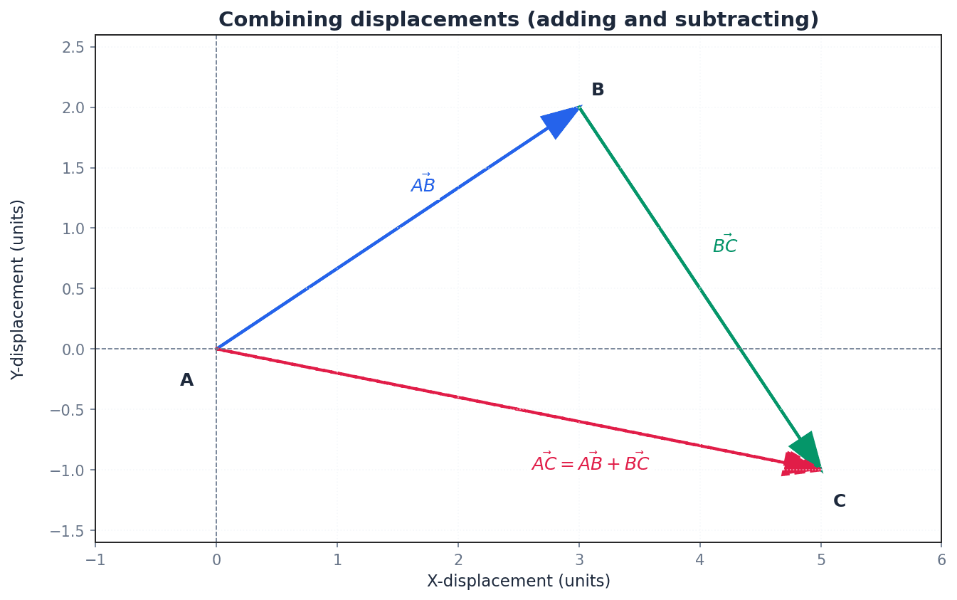
resultant vector — The overall displacement vector obtained by combining multiple displacement vectors.
When two or more vectors are added, the single vector that represents their combined effect is called the resultant vector. It describes the net change in position or force. For instance, if you walk 3m east and then 4m north, your resultant displacement vector is the single straight line from your start to end point.
Students often confuse displacement with distance; displacement is a vector (magnitude and direction), while distance is a scalar (magnitude only).
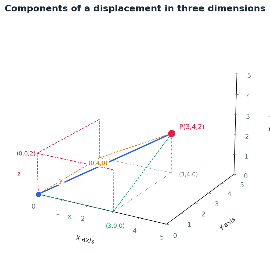
Vectors in two and three dimensions are represented using standard notation, either as column vectors or in i, j, k form. For example, a 3D vector can be written as (x, y, z) or xi + yj + zk. These components describe the displacement along the x, y, and z axes respectively.
Vectors can be added and subtracted by combining their corresponding components. Geometrically, vector addition follows the triangle rule, where vectors are placed head-to-tail to find the resultant. Multiplying a vector by a scalar changes its magnitude and can reverse its direction if the scalar is negative, but it does not change its fundamental direction.
Vector addition
Used to find the resultant displacement when vectors are added head-to-tail. This operation is commutative.
When finding a resultant vector, ensure you add corresponding components (x with x, y with y, z with z) correctly, especially when dealing with negative components.
magnitude — The length of the line segment representing the vector.
The magnitude of a vector, also known as its modulus, represents its size or length. It is calculated using Pythagoras' theorem based on its components. For example, if a car travels 50 km/h, 50 km/h is the magnitude of its velocity, regardless of the direction it's travelling.
modulus — The length of the line segment representing the vector.
The modulus of a vector is another term for its magnitude, indicating its size or length. It is a scalar quantity and is always non-negative. The absolute value of a number is like its modulus; it tells you its size regardless of its sign.
Magnitude of a 2D vector
Applies Pythagoras' theorem to find the length of a vector in two dimensions.
Magnitude of a 3D vector
Applies Pythagoras' theorem to find the length of a vector in three dimensions.
Students often think magnitude can be negative, but actually magnitude is always a non-negative scalar value, representing a length.
Always use Pythagoras' theorem for magnitude calculations, ensuring you square each component and sum them before taking the square root. For 3D vectors, include all three components.
unit vector — Any vector of magnitude or length 1.
A unit vector indicates a specific direction without conveying any magnitude beyond unity. It is found by dividing a vector by its own magnitude. A compass needle points in a direction (e.g., North) but doesn't tell you how far to go; it's a unit direction indicator.
Unit vector
Used to find a vector of length 1 in the same direction as a given vector.
Students often think a unit vector changes the direction of the original vector, but actually it only normalizes its length to 1 while preserving its original direction.
To find a unit vector in the direction of 'a', calculate |a| first, then divide each component of 'a' by |a|. The notation is 'a hat' (â).
position vector — A means of locating a point in space relative to an origin, usually O.
Unlike free displacement vectors, a position vector is fixed in space, always starting from a designated origin (often O) and ending at a specific point. It uniquely identifies the location of that point. Your home address is a position vector; it tells you exactly where your house is relative to a fixed reference point (like the city center).
free vectors — Displacement vectors that are not fixed to any particular starting point or origin.
Free vectors represent a displacement or translation that can occur anywhere in space. Many different arrows can represent the same free vector as long as they have the same magnitude and direction. A 'move forward 5 steps' instruction is a free vector; you can start from anywhere and move 5 steps forward.
Displacement vector between two points
Used to find the vector representing the displacement from point A to point B, given their position vectors relative to an origin O.
Students often think position vectors are the same as displacement vectors, but actually position vectors are fixed to an origin, while displacement vectors (free vectors) can represent the same movement anywhere in space.
When working with position vectors, remember that OA represents the vector from the origin O to point A. To find the displacement vector AB, use b - a.
A line in 2D or 3D space can be defined by a vector equation. This equation requires a position vector of a known point on the line and a direction vector parallel to the line. By varying a scalar parameter, any point on the line can be generated.
Vector equation of a line (point and direction)
Used to define a line in 2D or 3D space given a point on the line and a vector parallel to it.
Vector equation of a line (two points)
Used to define a line in 2D or 3D space given two points on the line. (c - a) forms the direction vector.
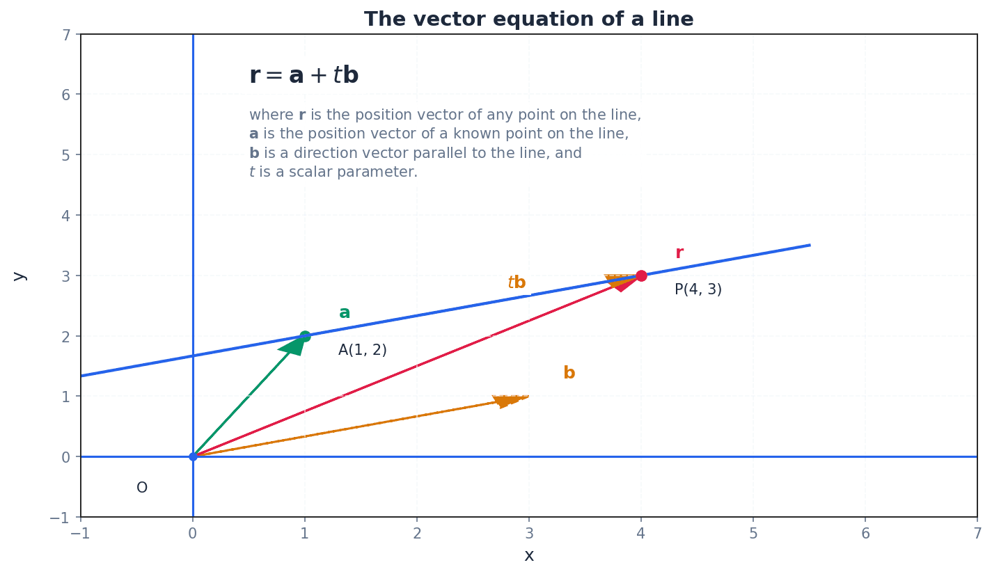
parametric equations — A set of equations that express the coordinates of points on a line in terms of a single variable parameter.
For a line, the parametric equations express x, y, and z coordinates as functions of a parameter (e.g., t). This allows any point on the line to be generated by varying the parameter. Think of a train schedule: the parameter 'time' determines the train's position (x, y, z coordinates) along its track.
Parametric equations of a line
Derived from the vector equation of a line, expressing each coordinate as a function of the parameter t. Useful for finding intersections.
When finding the point of intersection of two lines, converting their vector equations into parametric form is often the first step to equate corresponding components and solve for the parameters.
In three dimensions, two lines can be parallel, intersect at a single point, or be skew. Parallel lines have direction vectors that are scalar multiples of each other. Intersecting lines will have a common point, found by equating their parametric equations. Skew lines are non-parallel and do not intersect.
skew — Lines that are not parallel and do not intersect.
In 3-dimensional space, two lines are skew if they lie in different planes, are not parallel, and never meet. This is a unique concept to 3D geometry. Imagine two non-parallel roads, one passing over the other on a bridge without ever touching; they are skew.
Students often think non-parallel lines must intersect, but actually in 3D, they can be non-parallel and still not intersect if they are in different planes.
To prove lines are skew, first show they are not parallel (direction vectors are not scalar multiples). Then, attempt to solve their parametric equations simultaneously; if no consistent solution for the parameters exists, they are skew.
scalar product — A product of two vectors that gives an answer that is a scalar.
The scalar product (or dot product) of two vectors a and b is defined as a ⋅ b = |a||b|cosθ, where θ is the angle between them. It measures the extent to which two vectors point in the same direction. Imagine pushing a box: only the component of your force that is in the direction of the box's movement actually does 'work'. The scalar product quantifies this 'effective' force.
dot product — A product of two vectors that gives an answer that is a scalar.
The dot product is another name for the scalar product. It can be calculated geometrically using magnitudes and the angle between vectors, or algebraically by summing the products of corresponding components. It's like finding how much 'overlap' there is between two directions; if they're aligned, the overlap is maximal; if perpendicular, there's no overlap.
Geometric definition of scalar product
Used to calculate the scalar product when magnitudes and the angle between vectors are known, or to find the angle when the scalar product and magnitudes are known.
Algebraic definition of scalar product (component form)
Used to calculate the scalar product when the component forms of the vectors are known.
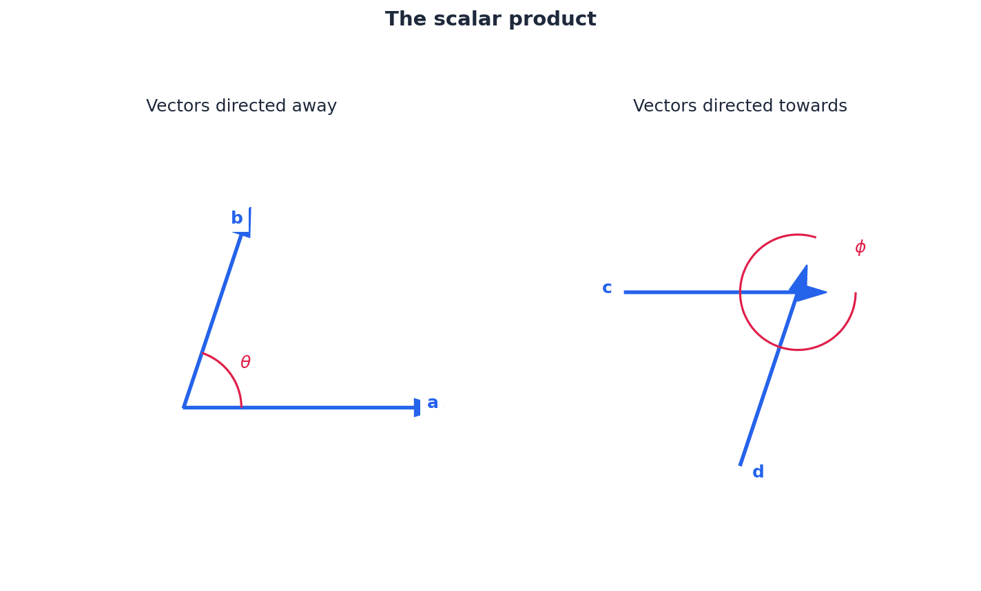
Students often think the scalar product results in a vector, but actually it always results in a single scalar number.
The scalar product is particularly useful for determining the relationship between two vectors. If two non-zero vectors are perpendicular, their scalar product is zero. If they are parallel, the angle between them is 0 or 180 degrees, and the scalar product simplifies to the product of their magnitudes (or negative product if opposite directions).
Remember that if two vectors are perpendicular, their scalar product is zero (a ⋅ b = 0). This is a crucial test for perpendicularity and a common exam question.
When finding the angle between two lines, students might use position vectors instead of the direction vectors of the lines.
vector product — A product of two vectors that gives an answer that is a vector.
The vector product (or cross product) of two vectors a and b results in a new vector perpendicular to both a and b. It is not required for Pure Mathematics 3. Imagine turning a wrench; the force you apply and the distance from the pivot create a torque, which is a vector quantity perpendicular to both.
cross product — A product of two vectors that gives an answer that is a vector.
The cross product is another name for the vector product. It is a binary operation on two vectors in three-dimensional space that results in a vector which is perpendicular to the plane containing the two input vectors. If you have two sticks on a table, their cross product would point straight up or straight down from the table.
For Pure Mathematics 3, you only need to know that the vector product exists but not how to calculate or use it. Focus on the scalar product.
Clearly state your vector notation (e.g., bold lowercase for vectors, uppercase for points) to avoid ambiguity.
Practice converting between vector and parametric forms of a line equation to ensure fluency.
Exam Technique
Finding the magnitude of a vector
Finding a unit vector in a given direction
| Mistake | Fix |
|---|---|
| Confusing displacement with distance. | Remember displacement is a vector (magnitude and direction), while distance is a scalar (magnitude only). |
| Assuming magnitude can be negative. | Magnitude is always a non-negative scalar value, representing a length. |
| Assuming non-parallel lines in 3D must intersect. | In 3D, lines can be non-parallel and still not intersect; these are called skew lines. |
This chapter introduces first order differential equations, which are fundamental for modelling rates of change in various real-world scenarios. Students will learn to formulate these equations from problem statements and solve them using the technique of separating variables, leading to general and particular solutions. The chapter also covers interpreting these solutions in context, including different growth models like exponential and logistic growth.
differential equation — An equation that has a derivative such as d/dx or d/dy as one of its terms is called a differential equation.
Differential equations describe how quantities change with respect to one another. They are fundamental in modelling real-world phenomena involving rates of change, such as population growth, cooling processes, or chemical reactions. Imagine a recipe that tells you how fast a cake bakes based on its current temperature; a differential equation is like that recipe, describing the rate of change rather than the final state.
first order differential equation — When the equation has the first derivative d/dx as one of its terms, it is called a first order differential equation.
This means the highest order derivative present in the equation is the first derivative. These are generally simpler to solve than higher-order differential equations and are commonly used to model immediate rates of change. If a differential equation is a recipe, a first order differential equation is a recipe that only tells you the immediate next step, not steps involving acceleration or further derivatives.
Students often think 'order' refers to the power of the derivative, but actually it refers to the highest derivative present (e.g., first derivative, second derivative).
Be careful to identify if the problem involves a first or higher order derivative, as the solution techniques differ. This chapter focuses exclusively on first order equations.
Differential equations are powerful tools for modelling real-world situations involving rates of change. The first step in solving such problems is to formulate the differential equation correctly from a problem statement. This involves translating descriptions of how quantities change, often involving proportionality, into derivative notation. For example, a rate of change being proportional to a quantity would be expressed as dP/dt = kP.
When asked to 'formulate' a differential equation, ensure you correctly translate the problem's language about rates of change and proportionality into derivative notation.
separating the variables — Separating the variables in the expression dy/dx = xy means that we are then able to integrate.
This technique involves rearranging a differential equation so that all terms involving y (and dy) are on one side of the equation, and all terms involving x (and dx) are on the other side. This allows for direct integration of both sides. It's like sorting laundry: putting all the 'y' clothes in one basket and all the 'x' clothes in another, so you can wash them separately.
Students often struggle with algebraic manipulation to separate variables, but actually careful rearrangement is key to making the equation integrable.
Practice algebraic manipulation to efficiently separate variables. Remember that constants can often stay on either side, but ensure all 'y' terms are with 'dy' and all 'x' terms with 'dx'.
general solution — The direct equation y = f(x) + C is called the general solution of the differential equation dy/dx = f'(x).
The general solution includes an arbitrary constant of integration, C, because integration is the reverse of differentiation, and the derivative of a constant is zero. This constant represents a family of possible solutions. If you know a car's speed, the general solution tells you all possible distances it could have travelled, differing only by its starting position (the constant C).
Forgetting to include the constant of integration 'C' when finding the general solution is a common error; this is a critical step that defines the family of solutions.
Always remember to add '+ C' when integrating to find the general solution. Marks are often awarded for its inclusion.
particular solution — To find a particular solution, we must have further information that will enable us to find the value of C.
A particular solution is obtained by using an initial condition (a specific point that the solution curve passes through) to determine the unique value of the constant of integration, C. This makes the solution specific to a given scenario. If the general solution is all possible distances a car could travel, the particular solution is the exact distance it travelled given its starting point.
Students often confuse the general and particular solutions, but actually the particular solution is a specific instance of the general solution, determined by an initial condition.
When an initial condition is provided, ensure you substitute the values into the general solution to find the constant C and present the final particular solution without C.
Once a differential equation has been solved, the resulting function needs to be interpreted within the context of the original problem. This involves understanding what the variables represent and how the mathematical solution describes the real-world phenomenon being modelled. For instance, a solution might describe how a population changes over time or how an object's temperature varies.
Students often think the solution to a differential equation is a number, but actually the solution is a function that describes the relationship between the variables.
Newton's Law of Cooling/Heating
Describes the rate of change of temperature of an object proportional to the difference in temperature between the object and its surroundings. The negative sign indicates cooling when T > Ts.
exponential growth — This type of growth is unlimited as the rate of growth of a population is proportional to the size of the population at that time.
In exponential growth, the rate of increase of a quantity is directly proportional to the quantity itself. This leads to a rapid, accelerating increase over time, often seen in early stages of population growth or compound interest. Imagine a snowball rolling down a hill, picking up more snow as it goes; the bigger it gets, the faster it grows.
Students often assume exponential growth can continue indefinitely, but actually in real-world scenarios, resources or space eventually become limited, leading to a different growth pattern.
logistic growth — A different model, logistic growth, can be used when resources are limited.
Logistic growth models a population whose growth rate decreases as it approaches a maximum capacity (carrying capacity) of its environment. The growth starts exponentially, then slows down, eventually levelling off. It's like a plant growing in a pot: it grows quickly at first, but as it fills the pot and uses up nutrients, its growth slows down.
Students often confuse logistic growth with exponential growth, but actually logistic growth accounts for environmental limits, leading to an S-shaped curve, unlike the ever-increasing exponential curve.
Logistic Growth Model
Models population growth when resources are limited, showing that the growth rate decreases as the population approaches the carrying capacity k.
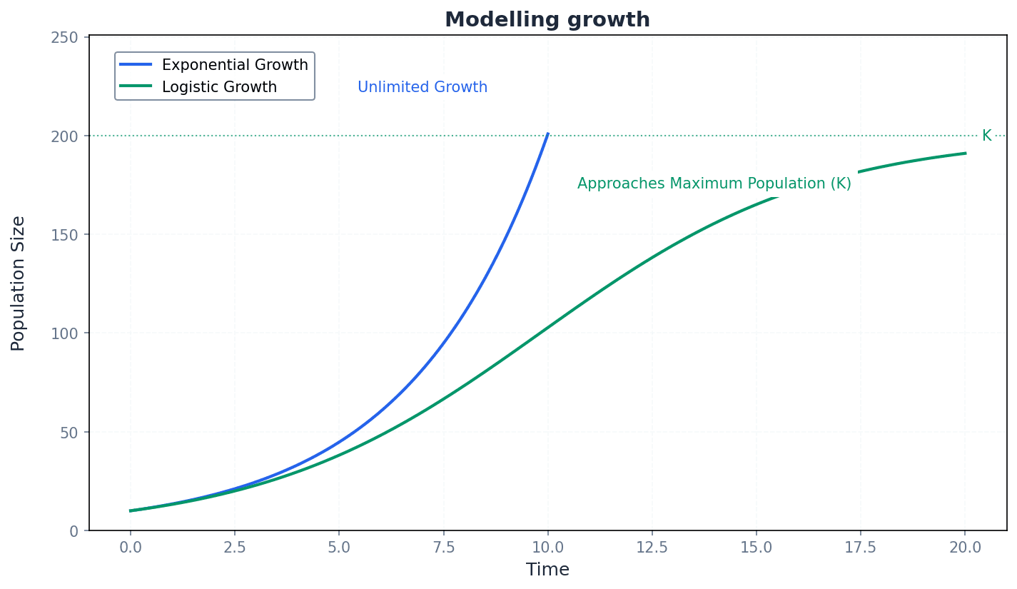
When interpreting logistic growth models, identify the carrying capacity (k) as the maximum population size the environment can sustain, which the population tends towards as time increases.
When interpreting solutions, relate the mathematical result back to the context of the problem being modelled.
Exam Technique
Solving a first order differential equation with separable variables
Modelling a real-world problem with a differential equation
| Mistake | Fix |
|---|---|
| Forgetting to include the constant of integration 'C'. | Always add '+ C' immediately after integrating to find the general solution. This is a critical step for full marks. |
| Confusing general and particular solutions. | Remember the general solution contains 'C', representing a family of curves. The particular solution is a specific curve found by using an initial condition to determine 'C'. |
| Incorrect algebraic manipulation when separating variables. | Practice rearranging equations carefully. Ensure all terms involving 'y' (and 'dy') are on one side and all terms involving 'x' (and 'dx') are on the other. Constants can often stay on either side. |
This chapter introduces complex numbers, which combine real and imaginary parts, and their representation on Argand diagrams. It covers arithmetic operations, conversion between Cartesian, modulus-argument, and exponential forms, and the use of complex conjugates. The chapter also explores solving polynomial equations with complex roots and illustrates simple equations and inequalities as loci.
Real number — The set of all rational and irrational numbers.
Real numbers are the numbers we have been working with until the introduction of imaginary numbers. They can be represented on a 1-dimensional number line, like all the points on a single, infinitely long ruler.
Imaginary number — Any multiple of the unit imaginary number i where i² is defined to be -1.
Imaginary numbers are of the form bi or yi, where b or y is a real number. They were introduced to solve equations that have no solutions in the set of real numbers, such as x² = -1. If real numbers are like movement along an east-west line, imaginary numbers are like movement along a perpendicular north-south line.
Definition of i
Fundamental definition of the unit imaginary number.
When simplifying expressions involving imaginary numbers, remember that i² = -1, i³ = -i, i⁴ = 1, and this cycle repeats. This is often tested in simplification questions.
Complex number — A number that can be written in the form x + yi where x and y are real values and i is the unit imaginary number.
Complex numbers extend the real number system by introducing an imaginary component, allowing solutions to equations like x² = -1. They are represented as points on a 2-dimensional plane, combining a real part and an imaginary part. Think of complex numbers like coordinates on a map (x, y), where x is your east-west position (real part) and y is your north-south position (imaginary part). You need both to specify a unique location.
When asked to define a complex number, ensure you explicitly state that x and y are real values and that i is the unit imaginary number where i² = -1.
Cartesian form — A complex number written as x + yi, where x and y are real values.
This form directly corresponds to Cartesian coordinates (x, y) on an Argand diagram, where x is the real part and y is the imaginary part. It is the standard way to express complex numbers for addition and subtraction. It's like giving directions by saying 'go 3 units east and 2 units north' (3 + 2i), directly specifying the horizontal and vertical components.
Students often think 'iy' is the imaginary part of z, but actually the imaginary part is the real number 'y', the coefficient of 'i'.
Complex number in Cartesian form
x and y are real values.
Equality of complex numbers
Two complex numbers are equal if and only if their real parts are equal and their imaginary parts are equal.
Operations of addition, subtraction, multiplication, and division can be carried out with complex numbers in Cartesian form. Addition and subtraction involve combining the real parts and imaginary parts separately. Multiplication uses the distributive law, remembering that i² = -1. Division typically involves the use of the complex conjugate to make the denominator a real number.
Complex conjugate — The complex conjugate of a complex number x + yi is defined as x - yi.
It is formed by changing the sign of the imaginary part of the complex number. Multiplying a complex number by its conjugate always results in a real number, which is useful for division. If a complex number is like a mirror image across the real axis, its conjugate is the reflection. They are symmetrical.
Students often think the complex conjugate changes the sign of both the real and imaginary parts, but actually only the sign of the imaginary part is changed.
Complex conjugate
Also denoted as \bar{z}.
Product of a complex number and its conjugate
The result is always a real number.
Complex numbers can be represented geometrically using an Argand diagram, which is a 2-dimensional plane where the horizontal axis represents the real part and the vertical axis represents the imaginary part. Each complex number z = x + yi corresponds to a unique point (x, y) or a position vector from the origin to (x, y). This visual representation helps in understanding the properties and operations of complex numbers.
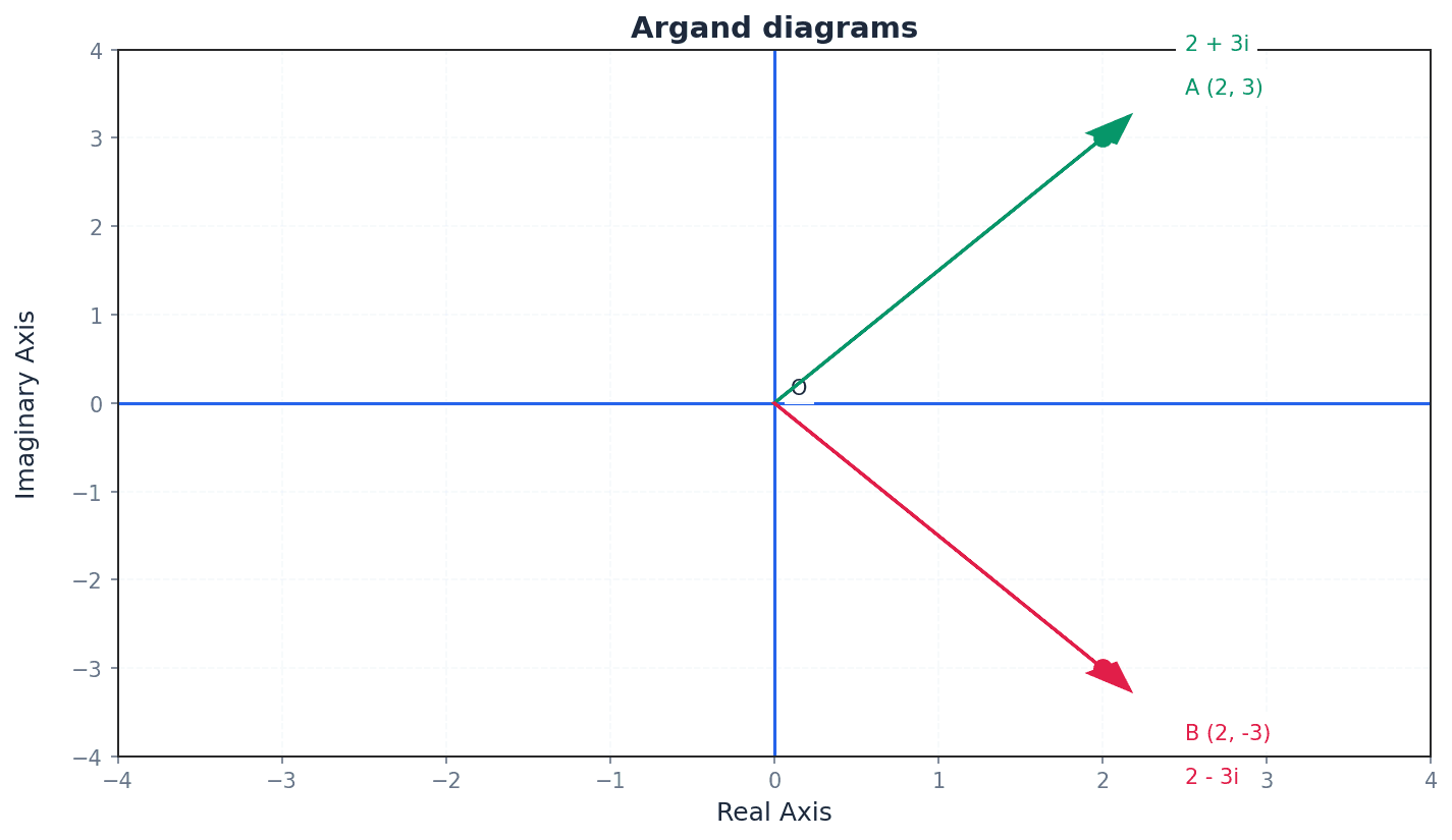
Modulus of a complex number — The modulus of a complex number x + yi is the magnitude of the position vector representing it on an Argand diagram.
It is defined as √(x² + y²) and represents the distance of the complex number from the origin in the complex plane. The plural of modulus is moduli. If a complex number is a point on a map, its modulus is the straight-line distance from the origin (your starting point) to that point.
Students often think the modulus can be negative, but actually it represents a distance and is always a non-negative real number.
When calculating the modulus, ensure you square both the real and imaginary parts before adding and taking the square root; do not include 'i' in the calculation.
Modulus of a complex number
Represents the magnitude of the position vector on an Argand diagram.
Argument of a complex number — The argument of a complex number x + yi is the direction of the position vector representing it on an Argand diagram.
More precisely, it is the angle made between the positive real axis and the position vector, usually given in radians. The principal argument, θ, is typically defined such that -π < θ ≤ π. If a complex number is a point on a radar screen, its argument is the bearing or direction from the center of the screen to that point.
Students often think the argument is always found using tan⁻¹(y/x), but actually a diagram must be drawn first to determine the correct quadrant and adjust the angle accordingly, especially for numbers in the second or third quadrants.
Always sketch an Argand diagram when finding the argument to correctly identify the quadrant and ensure the principal argument (-π < θ ≤ π) is given, usually in radians unless specified otherwise.
Students often confuse the principal argument range (-π < θ ≤ π) and other possible ranges (e.g., 0 ≤ θ < 2π) and must ensure they provide the argument in the specified range.
Argument of a complex number (acute angle)
Used to find the reference angle for the argument; a diagram is necessary to determine the correct quadrant.
Complex numbers can also be expressed in modulus-argument form, z = r(cosθ + isinθ), where r is the modulus and θ is the argument. This form is particularly useful for multiplication and division. Euler's formula, cosθ + isinθ = e^(iθ), allows for a concise exponential form, z = re^(iθ), which simplifies these operations even further.
Complex number in modulus-argument form (polar form)
r is the modulus and \theta is the argument.
Euler's formula
Relates trigonometric functions to the exponential function.
Complex number in exponential form (polar form)
r is the modulus and \theta is the argument.
Ensure you can convert between Cartesian form and polar/exponential forms, as questions often require answers in a specific format or involve operations that are easier in one form than another.
Multiplication of complex numbers in polar form
Multiply the moduli and add the arguments.
Division of complex numbers in polar form
Divide the moduli and subtract the arguments.
Complex numbers allow us to find solutions to polynomial equations that have no real roots, such as quadratic equations with a negative discriminant. A crucial result for solving higher-order polynomial equations with real coefficients is that non-real roots always occur in conjugate pairs. This means if x + yi is a root, then x - yi must also be a root.
Students often forget that for polynomial equations with real coefficients, non-real roots always occur in conjugate pairs, which is crucial for finding all roots.
Remember that for polynomial equations with real coefficients, non-real roots always occur in conjugate pairs. This is a crucial result for solving higher-order polynomial equations.
To find the square roots of a complex number, one typically sets the square root equal to an unknown complex number (x + yi), squares both sides, and then equates the real and imaginary parts to form simultaneous equations. Solving these equations yields the values of x and y, thus providing the two square roots.
Locus — A path traced out by a point as it moves following a particular rule, expressed as an inequality or an equation.
In the context of complex numbers, loci are represented on an Argand diagram and can describe shapes like circles, half-lines, or perpendicular bisectors, depending on the given equation or inequality involving z. Imagine a robot moving according to a set of instructions; the path it draws on the floor is its locus.
Students often think a locus is just a single point, but actually it is a set of points that satisfy a given condition, forming a geometric shape.
Simple equations and inequalities involving complex numbers can be illustrated as loci on an Argand diagram. For example, |z| = r represents a circle centered at the origin with radius r, while |z - (a + bi)| = r represents a circle centered at (a, b) with radius r. Inequalities define regions, such as the interior or exterior of a circle. Half-lines and perpendicular bisectors can also be represented, showing the geometrical effects of operations.
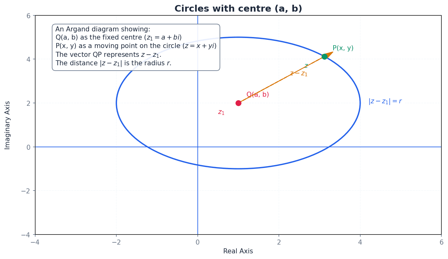
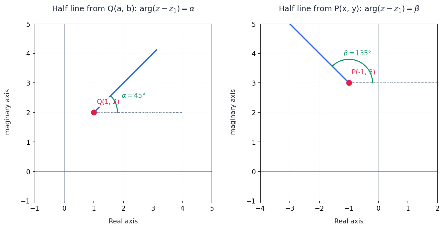
When sketching loci, pay close attention to whether the boundary is included (solid line) or not (dotted line) based on the inequality (≤, ≥ vs. <, >). Also, correctly identify the center and radius for circles, or the starting point and angle for half-lines.
Always draw an Argand diagram for loci questions to visualise the geometric interpretation of equations and inequalities.
Clearly label all parts of your Argand diagram, including axes, points, and loci, to gain full marks.
Exam Technique
Solving quadratic equations with complex roots
Finding modulus and argument of a complex number
| Mistake | Fix |
|---|---|
| Confusing 'iy' as the imaginary part. | Remember that the imaginary part is the real number 'y', the coefficient of 'i'. |
| Incorrectly calculating the argument using tan⁻¹(y/x) without considering the quadrant. | Always draw an Argand diagram first to determine the correct quadrant and adjust the angle accordingly (e.g., π - α for Q2, -π + α for Q3). |
| Stating a negative value for the modulus. | The modulus represents a distance and is always a non-negative real number. |
Generated by Nexelia Academy · nexeliaacademy.com