Pure Mathematics 2 & 3 · Algebra
This chapter covers the modulus function, including its definition, graphical representation, and methods for solving related equations and inequalities. It also introduces polynomial division, the factor theorem, and the remainder theorem, which are essential tools for factorising and solving cubic and quartic polynomial equations.
modulus — The modulus of a number is the magnitude of the number without a sign attached.
Also known as the absolute value, the modulus of any number (positive or negative) is always a positive number. For example, the modulus of 3 is 3, and the modulus of -3 is also 3. Think of the modulus as the 'distance from zero' on a number line. Whether you go 3 units to the right (positive) or 3 units to the left (negative), the distance covered is always 3 units.
absolute value — The modulus of a number is also called the absolute value.
This term is synonymous with 'modulus' and refers to the non-negative numerical value of a number, disregarding its sign. It is commonly denoted by vertical bars, e.g., |x|. If you're measuring the length of something, you always get a positive value, regardless of its orientation. The absolute value is like that 'length' of a number.
polynomial — A polynomial is an expression of the form a_n x^n + a_{n-1} x^{n-1} + … + a_1 x + a_0, where x is a variable, n is a non-negative integer, the coefficients a_0, a_1, ..., a_n are constants, a_n is called the leading coefficient and a_n ≠ 0, and a_0 is called the constant term.
Polynomials are fundamental algebraic expressions built from variables and coefficients using only addition, subtraction, multiplication, and non-negative integer exponents of the variable. The highest power of x in the polynomial determines its degree. Think of a polynomial as a 'recipe' for a function, where you combine different powers of x (like different ingredients) with specific constant amounts (coefficients) to create a mathematical expression.
leading coefficient — In a polynomial a_n x^n + a_{n-1} x^{n-1} + … + a_1 x + a_0, a_n is called the leading coefficient and a_n ≠ 0.
The leading coefficient is the coefficient of the term with the highest degree in a polynomial. It plays a crucial role in determining the end behaviour of the polynomial's graph. In a race, the 'leading runner' is the one at the front. Similarly, the leading coefficient is the number 'in front' of the highest power of x in a polynomial.
constant term — In a polynomial a_n x^n + a_{n-1} x^{n-1} + … + a_1 x + a_0, a_0 is called the constant term.
The constant term in a polynomial is the term that does not contain any variable, essentially the coefficient of x^0. It represents the y-intercept of the polynomial's graph. It's like the 'base cost' in a pricing formula – it's a fixed value that doesn't change regardless of the quantity (x) you buy.
degree of the polynomial — The highest power of x in the polynomial is called the degree of the polynomial.
The degree of a polynomial is a non-negative integer that indicates the highest exponent of the variable in any term of the polynomial. It helps classify polynomials (e.g., linear, quadratic, cubic) and influences the number of roots and the shape of its graph. Think of the degree as the 'level' of the polynomial. A higher degree means a more complex shape for its graph, just like a higher level in a game means more complexity.
dividend — In polynomial division, the dividend is the polynomial being divided.
When performing algebraic long division, the dividend is the polynomial that is 'inside' the division symbol. It is expressed as dividend = divisor × quotient + remainder. If you're sharing a cake, the whole cake is the dividend – it's what's being divided among people.
divisor — In polynomial division, the divisor is the polynomial by which another polynomial is divided.
The divisor is the polynomial that 'divides into' the dividend. If the remainder is zero, the divisor is a factor of the dividend. Continuing the cake analogy, the divisor is the number of people you're sharing the cake with – it's what you're dividing by.
quotient — In polynomial division, the quotient is the result of the division, excluding any remainder.
The quotient is the polynomial obtained when the dividend is divided by the divisor. It represents how many times the divisor 'fits into' the dividend. If you divide 10 by 3, the quotient is 3 – it's the whole number result of the division.
remainder — In polynomial division, the remainder is the polynomial left over after the division process, which has a degree less than the divisor.
The remainder is what is 'left over' after dividing one polynomial by another. If the remainder is zero, the divisor is a factor of the dividend. The remainder theorem provides a shortcut to find this value for linear divisors. If you divide 10 by 3, the remainder is 1 – it's what's left over after you've taken out as many whole groups of 3 as possible.
factor — If a polynomial P(x) divides exactly by a linear factor (x - c) to give the polynomial Q(x), then (x - c) is a factor of P(x).
A factor of a polynomial is an expression that divides the polynomial evenly, resulting in a remainder of zero. The factor theorem provides a direct way to test if a linear expression is a factor. In numbers, 2 is a factor of 6 because 6 divided by 2 leaves no remainder. Similarly, in polynomials, a factor divides without leaving a remainder.
factor theorem — If for a polynomial P(x), P(c) = 0, then (x - c) is a factor of P(x).
This theorem provides a quick method to determine if a linear expression (x - c) is a factor of a polynomial P(x) by simply evaluating P(x) at x = c. If the result is zero, then (x - c) is a factor. It's like a 'key test' for a lock. If you put the key (c) into the lock (P(x)) and it 'opens' (equals zero), then that key is a factor of the lock.
remainder theorem — If a polynomial P(x) is divided by (x - c), the remainder is P(c).
This theorem states that when a polynomial P(x) is divided by a linear divisor (x - c), the remainder of that division is equal to the value of the polynomial when x is replaced by c. It's a generalization of the factor theorem. Imagine you're trying to guess how much 'leftover' you'll have after sharing. The remainder theorem tells you that if you just 'try out' the sharing amount (c) in the original recipe (P(x)), you'll get the leftover directly.
x-intercept — The x-intercept is the point where the graph meets the x-axis.
At the x-intercept, the y-coordinate of the point is always zero. For a function y = f(x), the x-intercepts are the solutions to the equation f(x) = 0, also known as the roots of the equation. Imagine a car driving across a road. The x-intercept is where the car crosses the main road (the x-axis).
y-intercept — The y-intercept is the point where the graph meets the y-axis.
At the y-intercept, the x-coordinate of the point is always zero. For a function y = f(x), the y-intercept is found by evaluating f(0). Continuing the car analogy, the y-intercept is where the car crosses a side road (the y-axis).
vertex — The vertex of a modulus function graph of the form y = |ax + b| is the point where the graph changes direction, forming a 'V' shape.
For a modulus function y = |f(x)|, the vertex occurs where f(x) = 0. This is the point where the reflection in the x-axis takes place, resulting in the sharp turn of the graph. Think of the vertex as the 'hinge' of a folding ruler. It's the point where the two parts of the graph meet and change direction.
intersection — An intersection point is a point where two or more graphs meet.
The coordinates of an intersection point satisfy the equations of all the graphs that pass through it. Finding intersection points is a common method for solving simultaneous equations or inequalities graphically. Imagine two roads crossing each other. The point where they cross is their intersection.
inequality — An inequality is a mathematical statement that compares two expressions using an inequality symbol (e.g., <, >, ≤, ≥).
Solving an inequality means finding the range of values for the variable that makes the statement true. For modulus inequalities, this often involves considering different cases or interpreting graphs. Think of an inequality as setting a 'boundary' or a 'limit'. For example, x > 5 means x must be greater than 5, not just equal to it.
Modulus of x
Defines the modulus (absolute value) of a number.
Modulus equation property 1
Used to solve equations of the form |ax + b| = c, where 'a' is a positive constant.
Modulus equation property 2
Used to solve equations of the form |ax + b| = |cx + d|. This can also be written as ax + b = ±(cx + d).
Modulus inequality property 1
Used to solve modulus inequalities where the modulus is less than a positive constant.
Modulus inequality property 2
Used to solve modulus inequalities where the modulus is greater than a positive constant.
Division algorithm for polynomials
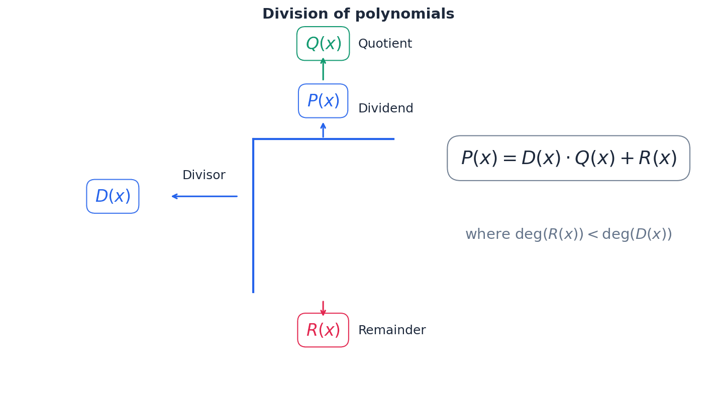
Relates the dividend P(x), divisor D(x), quotient Q(x), and remainder R(x) in polynomial division. The degree of the remainder R(x) must be less than the degree of the divisor D(x).
The modulus function, also known as the absolute value, gives the magnitude of a number without its sign. It is defined as |x| = x if x ≥ 0, and |x| = -x if x < 0. This means the output of a modulus function is always a non-negative value. For example, |3| = 3 and |-3| = 3.
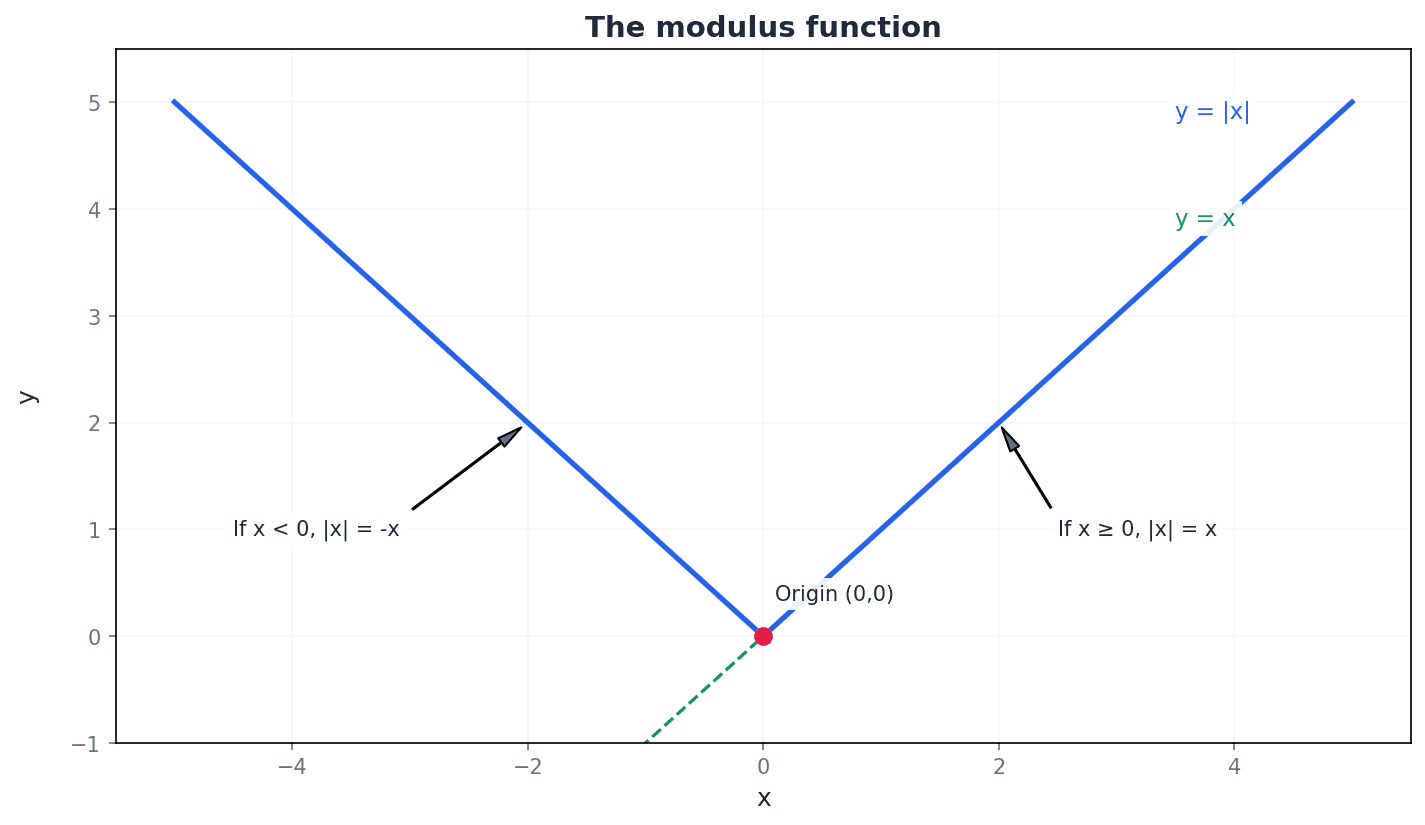
Students often think that |x| can be negative, but actually the modulus function always returns a non-negative value.
To solve equations involving the modulus function, such as |ax + b| = c, we consider two cases: ax + b = c or ax + b = -c. For equations of the form |ax + b| = |cx + d|, squaring both sides, i.e., (ax + b)^2 = (cx + d)^2, is an effective method. It is crucial to check all solutions in the original equation, especially when squaring, as extraneous roots can arise.
When solving equations or inequalities involving modulus, remember to consider both the positive and negative cases of the expression inside the modulus. For example, |x| = a means x = a or x = -a.
Students often forget to check solutions for modulus equations of the form |ax + b| = cx + d, as extraneous roots can arise from squaring both sides.
The graph of a modulus function of the form y = |ax + b| or y = |f(x)| where f(x) is linear, forms a characteristic 'V' shape. This shape is created by reflecting the part of the graph of y = f(x) that lies below the x-axis, upwards across the x-axis. The vertex of this 'V' shape is located at the x-intercept of the original linear function, i.e., where ax + b = 0.
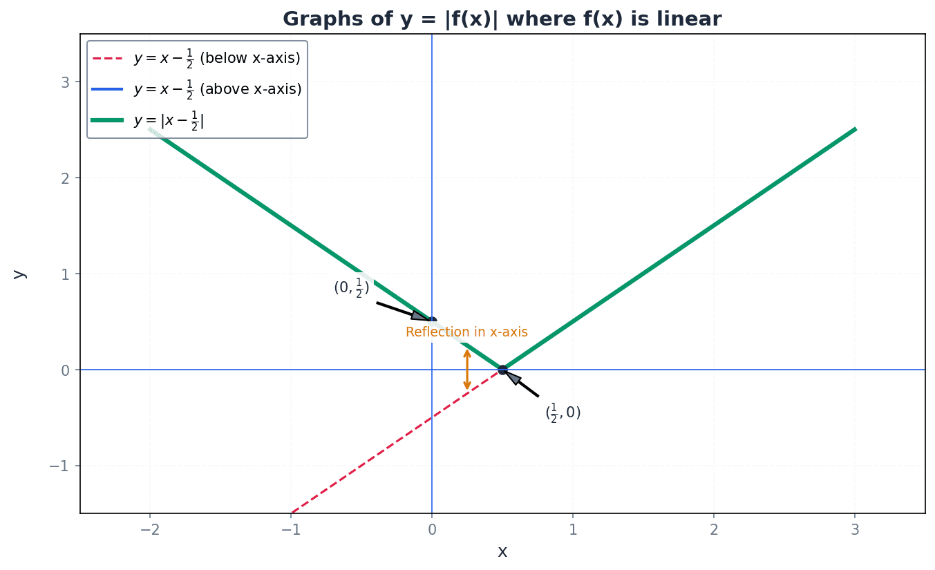
When sketching modulus graphs, accurately identifying and labelling the coordinates of the vertex is crucial for demonstrating understanding. Also, clearly label the coordinates of all x-intercepts and the y-intercept.
Students often think the vertex is always at the origin, but actually it depends on the linear function inside the modulus, i.e., where ax + b = 0.
Modulus inequalities can be solved algebraically by applying specific properties. For |x| < a, the solution is -a < x < a. For |x| > a, the solution is x < -a or x > a. Alternatively, graphical interpretation can be used by sketching the graphs of the functions involved and identifying the regions where the inequality holds true. Always check your solutions by substituting values from the determined range back into the original inequality.
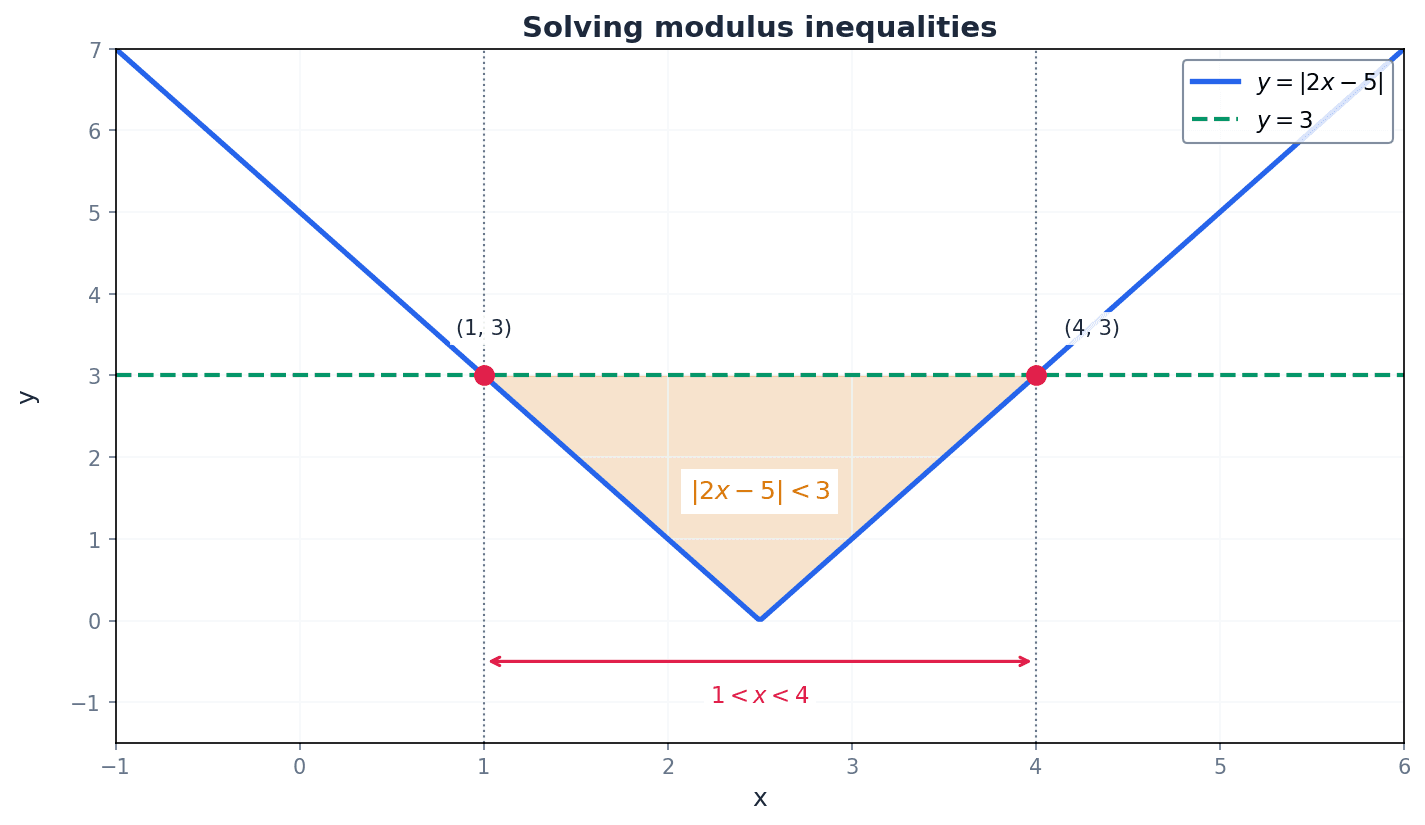
Students often confuse the conditions for modulus inequalities, e.g., using |x| > a for |x| < a, or vice versa. Remember that |x| < a means 'between' (-a < x < a), while |x| > a means 'outside' (x < -a or x > a).
Students often forget to reverse the inequality sign when multiplying or dividing by a negative number in algebraic manipulation.
Polynomial division is a method for dividing a polynomial (the dividend) by another polynomial (the divisor) to find a quotient and a remainder. The division algorithm for polynomials states P(x) = D(x)Q(x) + R(x), where the degree of the remainder R(x) must be less than the degree of the divisor D(x). This process is similar to numerical long division and is crucial for factorising and solving higher-degree polynomial equations.
Ensure you write the dividend in descending powers of x, including zero coefficients for any missing terms, to avoid errors in long division.
Students often forget to include zero coefficients for missing terms when performing polynomial long division, leading to incorrect alignment and calculations.
The Factor Theorem is a powerful tool stating that if P(c) = 0 for a polynomial P(x), then (x - c) is a factor of P(x). This allows for quick identification of linear factors. The Remainder Theorem generalizes this, stating that when a polynomial P(x) is divided by (x - c), the remainder is P(c). These theorems are invaluable for factorising and solving cubic and quartic polynomial equations by finding initial factors and reducing the polynomial to a quadratic.
The remainder theorem is a powerful tool for quickly finding the remainder when dividing by a linear factor (x - c) without performing full long division.
Students often confuse the factor theorem and the remainder theorem, or apply them incorrectly (e.g., testing P(c) for a factor (ax - b)). Remember the factor theorem is a special case of the remainder theorem where the remainder is zero.
For cubic and quartic equations, use the Factor Theorem to find initial factors, then use algebraic division or equating coefficients to find the remaining factors.
Students often fail to completely factorise polynomials, leaving quadratic factors that could be further broken down.
For modulus equations and inequalities, always consider both algebraic methods (squaring, definition) and graphical interpretation to verify solutions.
Method Frameworks
Common Errors
| Common mistake | How to fix it |
|---|---|
| Forgetting to consider both positive and negative cases when solving modulus equations or inequalities. | Always split modulus equations/inequalities into two distinct cases based on the definition of modulus, or by squaring both sides carefully. |
| Failing to check for extraneous roots when solving modulus equations of the form |ax + b| = cx + d by squaring. | After solving, substitute all potential solutions back into the original equation. Reject any solution that makes the right-hand side (cx + d) negative, as a modulus cannot equal a negative value. |
| Confusing the conditions for modulus inequalities (e.g., using |x| > a for |x| < a). | Remember: |x| < a means -a < x < a (values 'between'), and |x| > a means x < -a or x > a (values 'outside'). Visualise on a number line or graph if unsure. |
| Not including zero coefficients for missing terms in polynomial long division. | Before starting long division, write the dividend in descending powers of x, explicitly including terms with a coefficient of zero for any missing powers (e.g., x^3 + 0x^2 - 5x + 2). |
| Incorrectly applying the Factor or Remainder Theorem, especially with factors like (ax - b). | If the divisor is (x - c), evaluate P(c). If the divisor is (ax - b), evaluate P(b/a). The value to substitute is the root of the linear divisor. |
| Forgetting to reverse the inequality sign when multiplying or dividing by a negative number. | Make it a habit to explicitly check if you're multiplying or dividing by a negative number. If so, immediately reverse the inequality symbol. |
| Not fully factorising polynomials, leaving reducible quadratic factors. | After using algebraic division to reduce a polynomial to a quadratic, always attempt to factorise the quadratic further (using inspection, quadratic formula, or factorisation techniques) until all factors are linear or irreducible over real numbers. |
Technique Selection
| When you see... | Use... |
|---|---|
| Solving |ax + b| = c (where c is a constant) | Split into two linear equations: ax + b = c and ax + b = -c. |
| Solving |ax + b| = |cx + d| | Square both sides: (ax + b)^2 = (cx + d)^2. Alternatively, split into ax + b = (cx + d) and ax + b = -(cx + d). |
| Solving |ax + b| = cx + d (where cx + d is a variable expression) | Split into two linear equations: ax + b = cx + d and ax + b = -(cx + d). Crucially, check for extraneous roots by ensuring cx + d ≥ 0 for valid solutions. |
| Solving modulus inequalities like |ax + b| < c | Rewrite as a compound inequality: -c < ax + b < c. |
| Solving modulus inequalities like |ax + b| > c | Split into two separate inequalities: ax + b < -c or ax + b > c. |
| Solving modulus inequalities involving two modulus expressions, e.g., |ax + b| ≥ |cx + d| | Square both sides: (ax + b)^2 ≥ (cx + d)^2, then solve the resulting quadratic inequality. |
| Sketching graphs of y = |ax + b| | First, sketch y = ax + b. Then, reflect the part of the graph below the x-axis in the x-axis. Identify and label the vertex (where ax + b = 0) and intercepts. |
| Dividing a polynomial by a linear or quadratic polynomial (degree ≤ 4) | Use algebraic long division. Ensure all powers of x are represented in the dividend with zero coefficients if necessary. |
| Determining if (x - c) is a factor of P(x) | Apply the Factor Theorem: calculate P(c). If P(c) = 0, then (x - c) is a factor. |
| Finding the remainder when P(x) is divided by (x - c) | Apply the Remainder Theorem: calculate P(c). The value P(c) is the remainder. |
| Factorising or solving cubic/quartic polynomial equations | Use the Factor Theorem to find an initial linear factor (x - c). Then, use algebraic division to divide P(x) by (x - c) to obtain a quadratic (for cubic) or cubic (for quartic). Repeat for the cubic or factorise the quadratic. |
Mark Scheme Notes