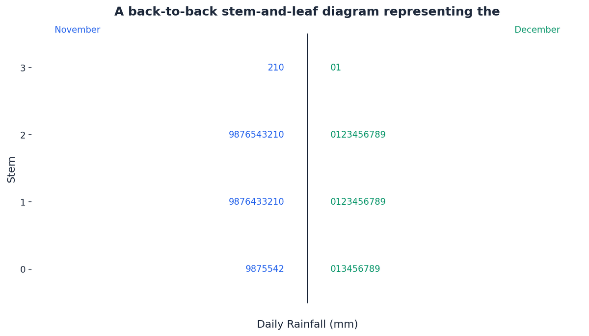
Fig 1.2 shows a back-to-back stem-and-leaf diagram representing the daily rainfall (mm) in a certain town for the months of November and December. (a) Find the number of days in November with rainfall less than 15 mm. (b) State the median daily rainfall for December.
A researcher is recording the ages of participants in a study. The ages are recorded as whole numbers. (a) For a continuous dataset, identify the lower and upper class boundaries for the interval 20-29. [2] (b) Calculate the frequency densities for the classes 10-19 (frequency 15) and 20-29 (frequency 25), assuming equal-width intervals based on the boundaries identified in part (a). [4]
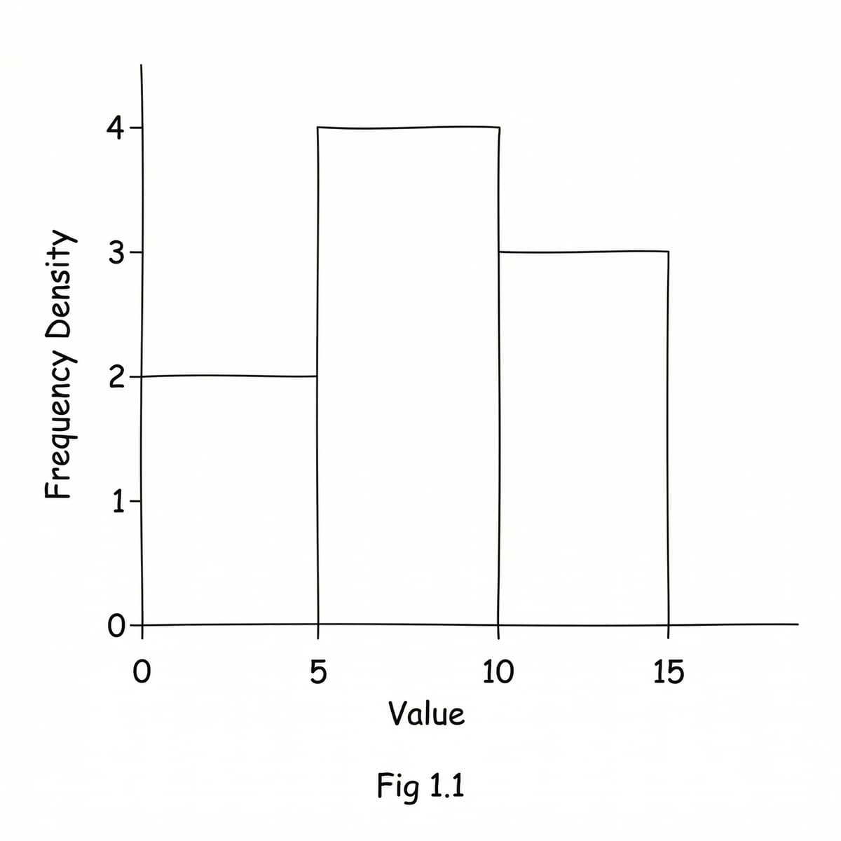
Fig 1.1 shows a histogram illustrating the race completion times for a group of athletes. (a) Determine the frequency of the class interval 10-15 seconds. [4] (b) Calculate the percentage of athletes who completed the race in less than 20 seconds. [4] (c) Comment on the shape of the distribution shown by the histogram. [2]
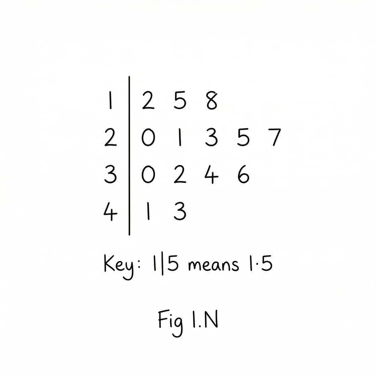
The lengths, in cm, of a sample of insects are shown in the stem-and-leaf diagram in Fig 1.1. Fig 1.1 Stem | Leaves ---- | ------ 1 | 2 5 8 2 | 0 1 3 5 7 3 | 0 2 4 6 4 | 1 3 Key: 1|5 means 1.5 cm (a) Calculate the range and interquartile range of the data represented in Fig 1.1. [4] (b) Interpret what the interquartile range indicates about the spread of the data. [3]
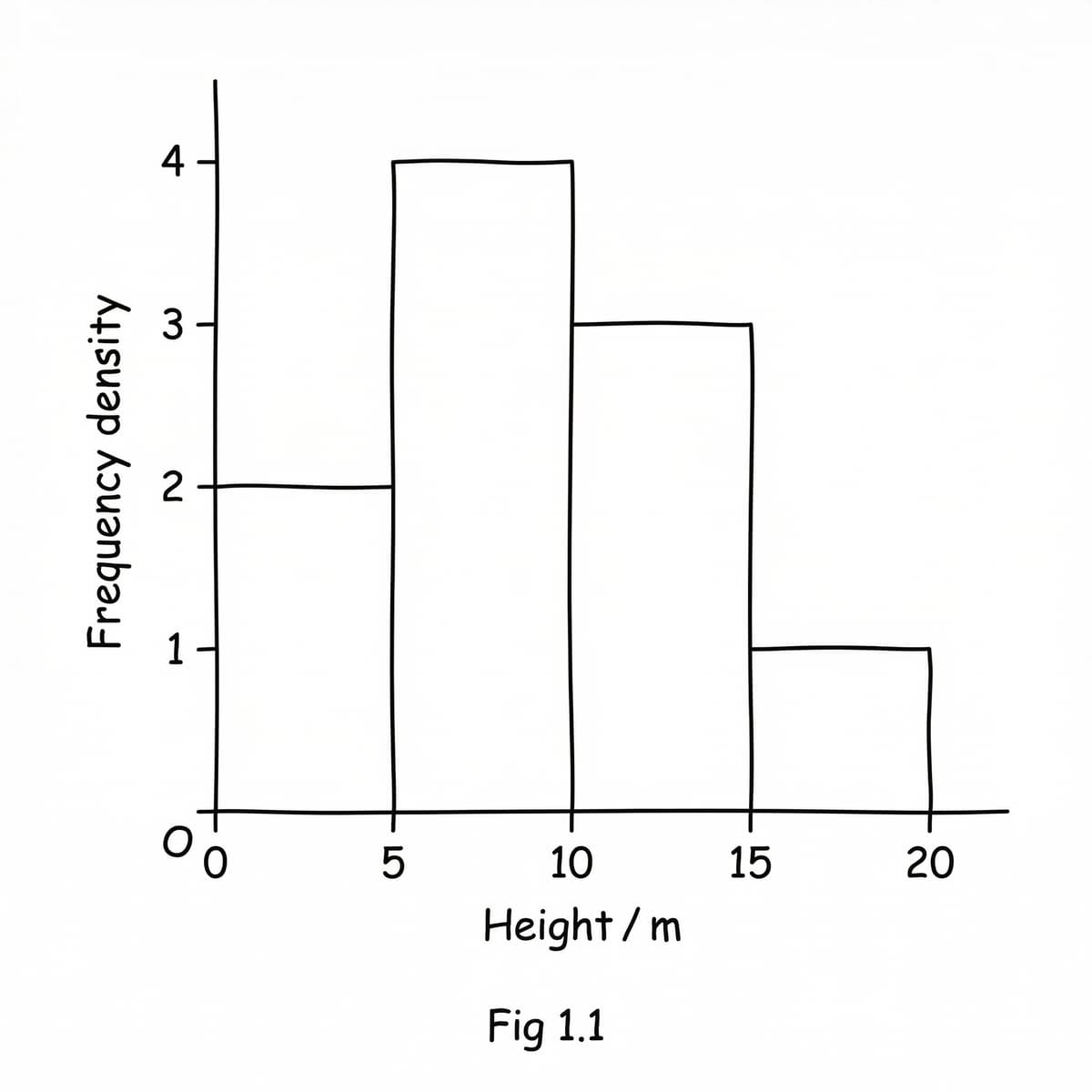
A conservation group measured the heights of trees in a small forest area. The data collected is presented in the histogram shown in Fig 1.1. Fig 1.1 (a) Interpret the information presented in the histogram regarding the distribution of tree heights. [4] (b) Estimate the number of trees with heights between 8m and 12m. [4]
A researcher is comparing the reaction times (in milliseconds) of two different groups of participants, Group X and Group Y, to a visual stimulus. (a) Construct a back-to-back stem-and-leaf diagram for the following two datasets: Group X: 12, 15, 18, 21, 22, 25, 27, 30, 31, 33 Group Y: 10, 14, 16, 19, 20, 23, 26, 28, 29, 32 [5] (b) Compare the two groups based on their medians and ranges from your diagram. [4]
Fig 1.3 shows a histogram representing the masses of a group of children. (a) Calculate the frequency density for the class interval 50-70 kg. [3] (b) Estimate the number of children with masses less than 40 kg. [3] (c) State why a histogram is a suitable representation for this data. [2]
The number of goals scored by two football teams, Team A and Team B, in 10 matches each, were recorded. Team A: 1, 3, 0, 2, 1, 4, 2, 3, 1, 0 Team B: 2, 1, 3, 0, 2, 5, 1, 4, 3, 2 (a) Construct a back-to-back stem-and-leaf diagram to compare the number of goals scored by the two teams. [6] (b) Compare the median number of goals for both teams using your diagram. [2]
Histograms are powerful tools for visualising continuous data, but their construction requires specific terminology and understanding. (a) Define the term 'frequency density' as it applies to histograms. [2] (b) Define what the area of a bar in a histogram represents. [2]
Data can be represented in various ways to highlight different characteristics. Both histograms and bar charts use bars to display frequencies. (a) State one key difference between a histogram and a bar chart. [2] (b) Explain why histograms are generally preferred for representing continuous data over bar charts. [3]
A study recorded the heights of 100 students, grouped into the following frequency distribution:
| Height (cm) | Frequency | |||
|---|---|---|---|---|
| 150-155 | 10 | \ | 155-160 | 25 |
| 160-165 | 40 | |||
| 165-170 | 20 | |||
| 170-175 | 5 |
(a) Draw a cumulative frequency curve for this distribution on a piece of graph paper. [5] (b) Using your curve, estimate the number of people shorter than 158 cm. [2] (c) Using your curve, find the height below which 70% of the people lie. [2]
Different types of data representation are suitable for different purposes. (a) Identify which data representation (stem-and-leaf diagram, histogram, or cumulative frequency graph) would be most suitable for each of the following scenarios, giving a brief reason: (i) showing individual data points for a small dataset. [2] (ii) illustrating the overall shape of a large continuous dataset. [2]
Fig 1.3 shows a histogram titled 'Production Output per Hour' representing the number of units produced per hour by a factory. (a) Calculate the frequency density for the class interval 100-150 units. (b) Estimate the total number of items produced that are represented in the histogram. (c) Explain why the class 0-50 units has the highest frequency density but not necessarily the highest frequency.
A regional car sales manager wants to compare the performance of two dealerships, Dealership A and Dealership B, over 15 months. The number of cars sold each month is recorded as follows: Dealership A: 21, 28, 30, 32, 35, 35, 37, 40, 41, 43, 45, 48, 50, 52, 55. Dealership B: 18, 20, 22, 25, 27, 29, 30, 31, 33, 36, 38, 40, 42, 44, 46. (a) Construct a back-to-back stem-and-leaf diagram for the number of cars sold by the two dealerships. [5] (b) Find the median for each dealership. [2] (c) Comment on the central tendency of sales for both dealerships based on your medians. [2]
Fig 1.2 shows a histogram representing the mathematics test scores of a group of students. (a) Calculate the total number of students represented in the histogram. [3] (b) Estimate the number of students who scored between 50 and 70 marks. [3] (c) Comment on the skewness of the distribution of test scores. [3]
Fig 1.2 shows a histogram representing the race times of a group of athletes. (a) Calculate the frequency density for the class interval 15.5-18.5 min. [3] (b) Determine the total number of athletes represented in the histogram. [3]
Histograms are a common way to represent continuous data. When constructing a histogram, the choice of interval widths is important. (a) Identify the primary advantage of using equal-width intervals when constructing a histogram. [2] (b) State the formula used to calculate frequency density for a histogram with equal-width intervals. [3]
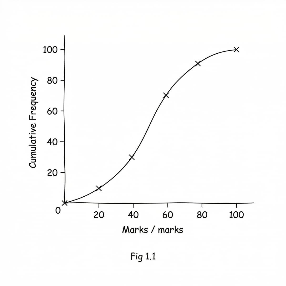
Fig 1.1 shows a cumulative frequency graph for the marks of 100 students in an exam. (a) Estimate the interquartile range from the graph. [3] (b) Calculate the number of students who scored between 50 and 70 marks. [4] (c) Explain why it is not possible to determine the exact mean from this graph. [3]
Different types of data require different methods of representation. Understanding the strengths of each representation is crucial for effective data analysis. (a) Name two types of data representation suitable for continuous data. [2] (b) Identify three pieces of information that can be easily obtained from a cumulative frequency graph but not directly from a stem-and-leaf diagram. [3]
Bar charts and histograms are often confused, but they serve different purposes in data representation. (a) Discuss the potential misinterpretations that could arise from using a bar chart instead of a histogram for continuous data. [5] (b) Suggest a scenario where a bar chart would be more appropriate than a histogram for representing numerical data. [3]
A teacher recorded the scores of 18 students in a recent mathematics test. (a) Construct a stem-and-leaf diagram for the following test scores: 65, 72, 81, 68, 75, 90, 62, 78, 85, 70, 73, 88, 60, 79, 83, 76, 92, 69. [4] (b) Calculate the mean test score from your diagram. [2] (c) Find the percentage of students who scored 80 or above. [2]
Different graphical representations are used to visualise continuous data, each with specific strengths. (a) Compare the effectiveness of a histogram versus a cumulative frequency graph for identifying the mode of a continuous dataset. [6] (b) Evaluate the strengths and weaknesses of using a histogram to represent a dataset with a very large range of values. [5]
A researcher collected data on the scores of participants in a cognitive task. The data is represented in the histogram shown in Fig 1.1. (a) Determine the frequencies for each class interval from the provided histogram. (i) For the interval 0-5. [1] (ii) For the interval 5-10. [1] (iii) For the interval 10-15. [1] (iv) State the total number of participants. [1] (b) Explain how you used the frequency density values to find the frequencies. [3]
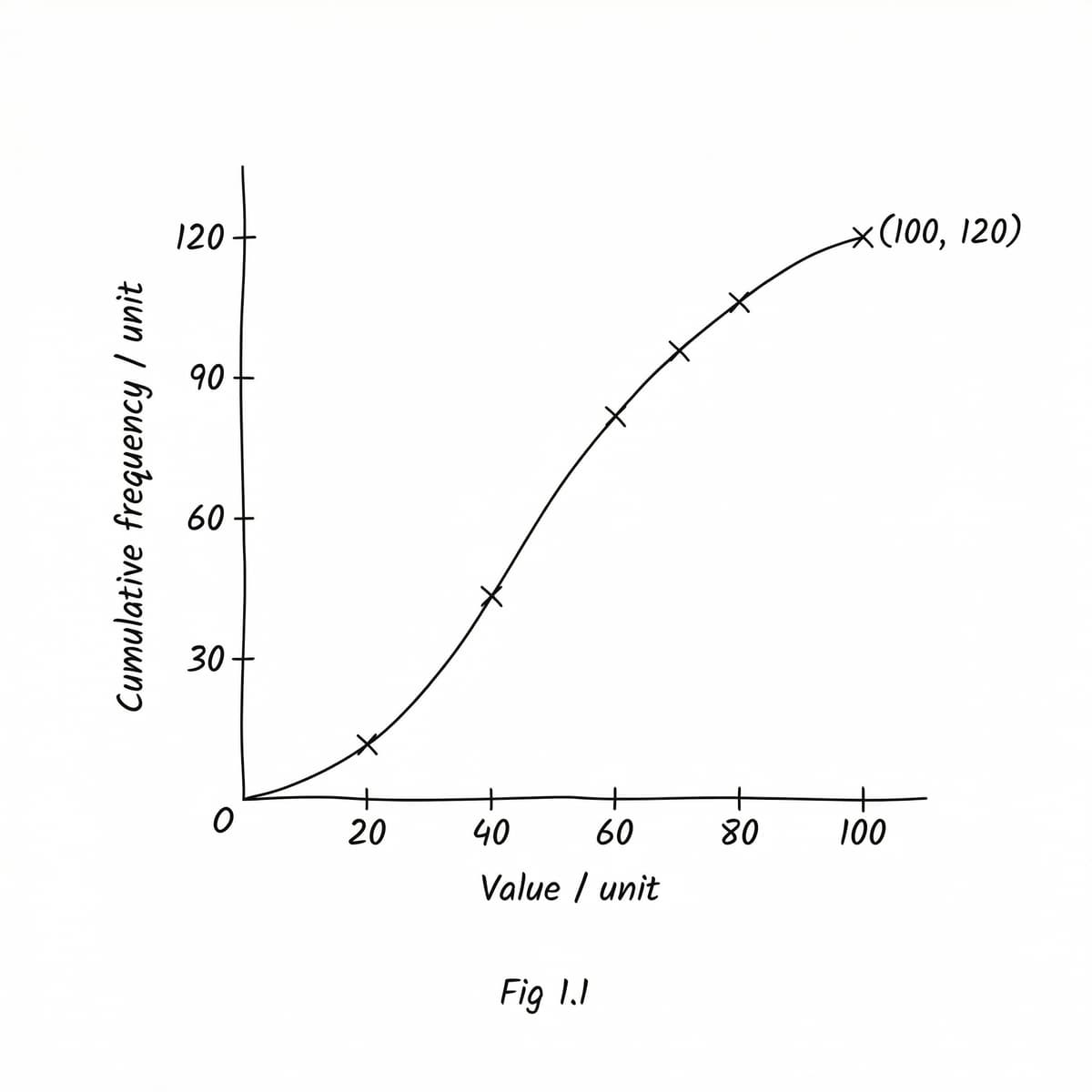
The cumulative frequency graph in Fig 1.1 shows the distribution of 120 measurements taken during an experiment. (a) Using the graph, calculate the frequency of the class 60-70. [5] (b) Estimate the percentage of data points that fall within the range 45 to 85. [3]
The table below shows the journey times, in minutes, for 50 commuters travelling to work.
| Journey time (min) | Frequency | |||
|---|---|---|---|---|
| 0-10 | 5 | |||
| 10-20 | 12 | \ | 20-30 | 18 |
| 30-40 | 10 | |||
| 40-50 | 5 |
(a) Construct a cumulative frequency graph for this data on a piece of graph paper. [6] (b) Using your graph, estimate the 10th percentile of journey times. [3] (c) Comment on the skewness of the distribution based on your graph. [2]
Histograms and stem-and-leaf diagrams are both effective ways to represent data, but they serve different purposes and have distinct characteristics. (a) Compare the advantages and disadvantages of using a histogram versus a stem-and-leaf diagram to represent data. [5] (b) Explain when a histogram would be preferred over a stem-and-leaf diagram. [3]
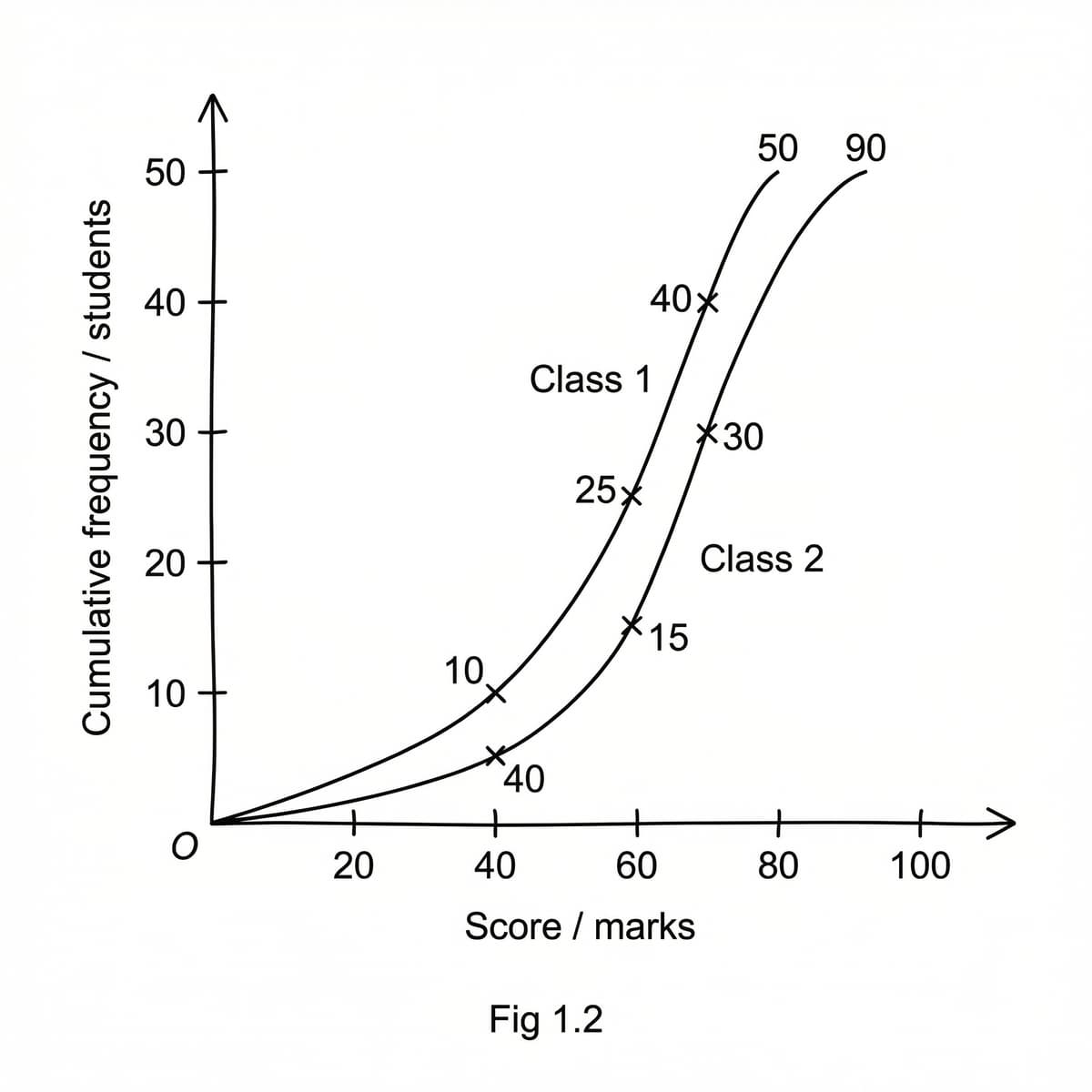
Fig 1.2 shows two cumulative frequency graphs, representing the scores of Class 1 and Class 2 in a mathematics test. There are 50 students in each class. (a) Determine the percentage of students who scored above 70 marks in each test. [4] (b) Explain which class performed better overall, justifying your answer using statistical measures from the graphs. [4]
Data representation choices are crucial for effective comparison and analysis. Different types of diagrams offer unique advantages and disadvantages depending on the nature and size of the dataset. (a) Discuss the strengths and weaknesses of using a cumulative frequency graph to compare two different datasets. [7] (b) Evaluate whether a back-to-back stem-and-leaf diagram or two separate cumulative frequency graphs would be more effective for comparing the ages of students in two different schools (one with 30 students, another with 200 students). [5]
Fig 1.2 shows a histogram representing the speeds of cars on a highway. (a) Calculate the total number of cars whose speeds are recorded. [3] (b) Determine the frequency of cars travelling between 40 km/h and 60 km/h. [3] (c) Explain why the height of the bar for 60-80 km/h is not directly proportional to the frequency for that class. [3]
In a study of daily commute times, data was collected for a group of employees and organised into class intervals for a histogram. (a) Calculate the frequency density for the class 15-20 minutes, given that the frequency for this class is 30 employees. [3] (b) Determine the class frequency for an interval with a class width of 10 minutes and a frequency density of 2.5 employees per minute. [4]
Different data representations are suitable for different types of data and purposes of analysis. (a) Describe one situation where a stem-and-leaf diagram is a more appropriate representation than a histogram. [3] (b) Give one advantage of using a histogram for a large dataset compared to a stem-and-leaf diagram. [3]
Fig 1.1 shows a histogram illustrating the volume of liquid distributed to a sample of containers. (a) Calculate the frequency of the class interval 10-20 litres. [3] (b) Determine the total volume of liquid distributed, assuming the mid-point of each class for calculation. [3] (c) Discuss why frequency density is used on the y-axis instead of frequency. [2]
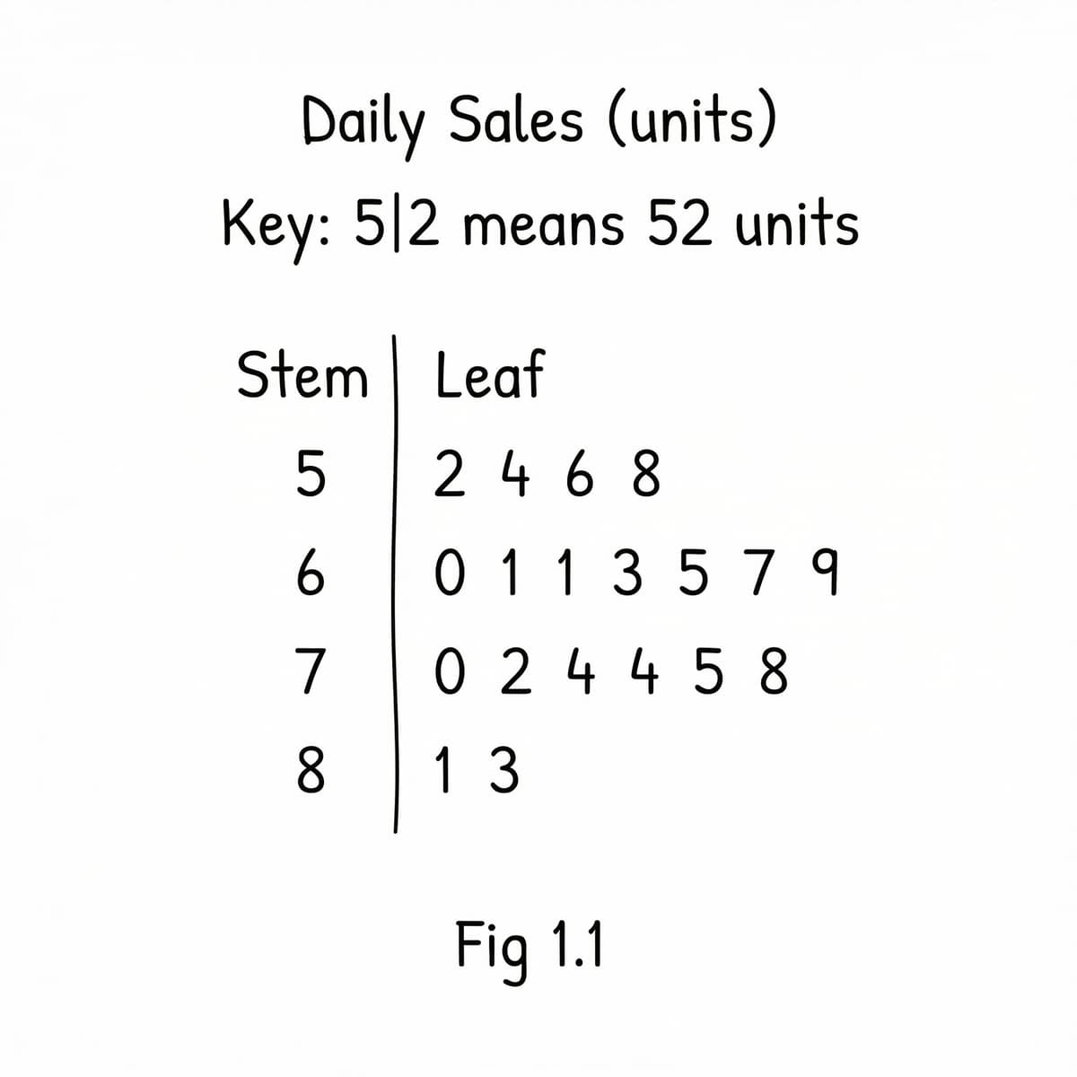
A retail store records the number of units sold each day over a period of time. The daily sales data is represented in the stem-and-leaf diagram shown in Fig 1.1. Fig 1.1 Daily Sales (units) Key: 5|2 means 52 units 5 | 2 4 6 8 6 | 0 1 1 3 5 7 9 7 | 0 2 4 4 5 8 8 | 1 3 (a) Discuss the strengths and limitations of using a stem-and-leaf diagram for representing large data sets compared to small data sets. [6] (b) Calculate the mean of the data set shown in Fig 1.1, ensuring you show your working. [5]
A study recorded the time taken for a new chemical reaction to complete, with the results displayed in the histogram in Fig 1.1. (a) Analyse the shape of the distribution shown in Fig 1.1, commenting on skewness and spread. [6] (b) Discuss the implications of this distribution for the variable being measured. [4]
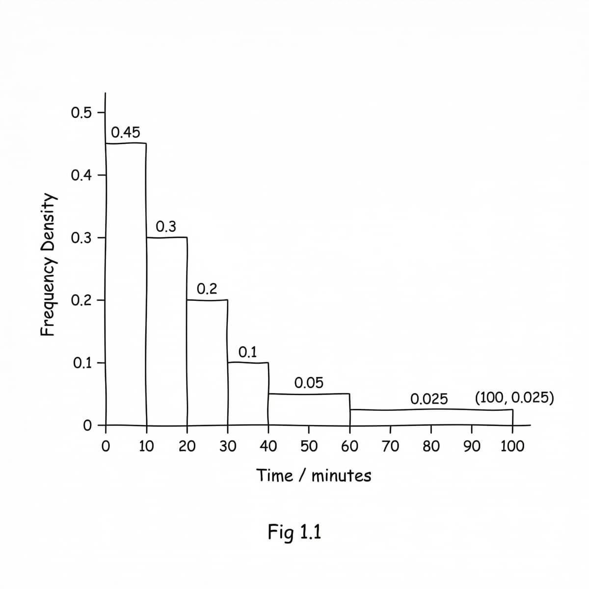
Fig 1.1 shows two cumulative frequency graphs, A and B, representing the heights of two different groups of plants. (a) Interpret the differences in the median values of the two datasets shown in Fig 1.1. [4] (b) Compare the spread of the two datasets using the interquartile range. [3]
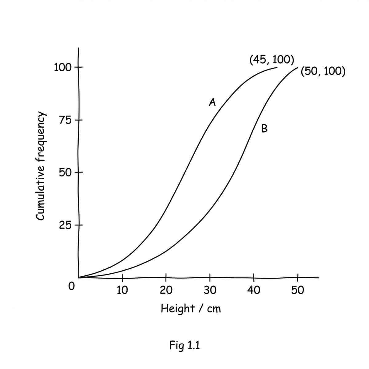
Fig 1.3 shows a histogram representing the duration of phone calls made from an office. (a) Calculate the frequency of the class 20-30 minutes. [3] (b) Estimate the proportion of calls that lasted longer than 40 minutes. [3] (c) Justify why there are no gaps between the bars in the histogram. [2]
Fig 1.2 shows a histogram representing the distribution of a continuous variable. (a) Describe the overall shape and spread of the data shown in the histogram in Fig 1.2. [4] (b) Suggest a possible real-world scenario that this distribution could represent, justifying your choice with reference to the characteristics identified in part (a). [4]
Fig 1.1 shows two histograms, P and Q, representing the test scores of two different classes in a recent examination. (a) Analyse the skewness of the distribution for both datasets based on the provided histograms. [5] (b) Discuss which representation (histogram or cumulative frequency graph) would be more suitable if the primary goal is to identify outliers and extreme values. [5]
Fig 1.4 shows a stem-and-leaf diagram representing the exam scores of a group of students. (a) Find the number of students who scored exactly 75 marks. [2] (b) State the highest score achieved by a student. [2]
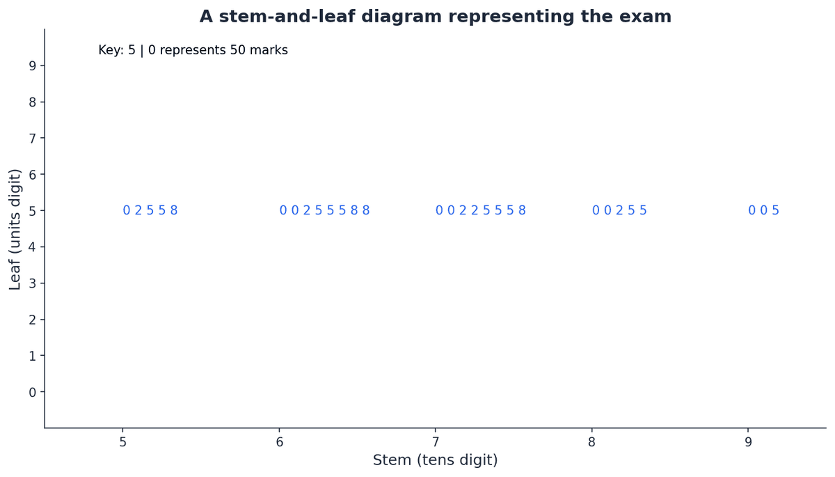
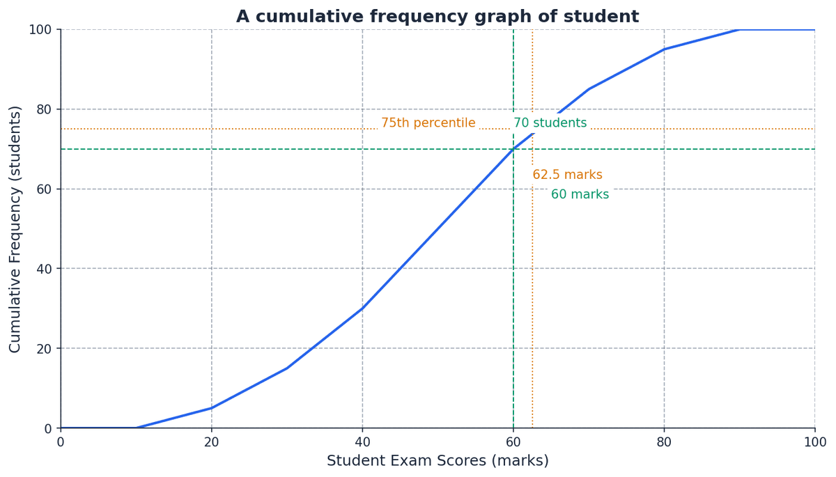
Fig 1.3 shows a cumulative frequency graph of student exam scores. (a) Estimate the number of students who scored less than 60 marks. [2] (b) Determine the 75th percentile score from the graph. [3]
Representation of data · Probability & Statistics 1
Upgrade to Pro to upload images of your work.